An Improved CBR Model Using Time-series Data for Predicting the End-point of a Converter - J-Stage
←
→
Page content transcription
If your browser does not render page correctly, please read the page content below
ISIJ International, Advance
                                      ISIJ Publication
                                           International,
                                                       by Advance
                                                           J-STAGE,Publication          ISIJ International, Vol. 61 (2021), No. 10, pp. 1–7
                                                                      DOI: 10.2355/isijinternational.ISIJINT-2020-687
                                                                                  by J-STAGE
     ISIJ International, J-Stage Advanced
                                       ISIJ International,
                                            Publication,
                                             ISIJ International,
                                                         DOI:
                                                           Advance
                                                              http://dx.doi.org/10.2355/isijinternational.ISIJINT-2015-@@@
                                                                 Vol. Publication
                                                                      61 (2021),  No.
                                                                                   by J-Stage
                                                                                       10
                                                                               https://doi.org/10.2355/isijinternational.ISIJINT-2020-687

An Improved CBR Model Using Time-series Data for Predicting
the End-point of a Converter

Mao-qiang GU, An-jun XU,* Fei YUAN, Xiao-meng HE and Zhi-feng CUI

School of Metallurgical and Ecological Engineering, University of Science and Technology Beijing, Beijing, 100083 China.
             (Received on November 15, 2020; accepted on June 1, 2021; J-STAGE Advance published date:
             August 26, 2021)

              The end-point temperature is one of parameters for the end-point control in the converter. Accurate
           prediction of the end-point temperature is helpful to improve the hit rate of the end-point. An improved
           CBR model using time-series data (CBR_TM) was proposed to predict the end-point carbon content and
           temperature in the converter according to the data types of process parameters. The attributes of the
           cases in the model not only include the influencing factors of single-value type such as composition and
           temperature of hot metal, but also include the influencing factors of time-series type such as lance posi-
           tion and oxygen flow, in the case retrieval process, the single-value data similarity and time-series data
           similarity between the cases were calculated based on the Euclidean distance and the dynamic time warp-
           ing algorithm, and then weighted to obtain the comprehensive similarity. Then the influence of the weight
           of the time-series data similarity on the prediction accuracy was studied based on the production data.
           Finally, the prediction accuracy of the established model was also compared to models based on SVR and
           BPNN. The results show that: The prediction accuracy of the model increases at first and then decreases
           with the increase of similarity weight of time series data. The prediction accuracy of the model was the
           highest when the weight of time-series data similarity was 0.4 and was better than the SVR and BPNN
           models. The established can meet the requirements of field production.

           KEY WORDS: end point prediction; case-based reasoning; time-series; dynamic time warping.

                                                                                such a model is comparatively ideal and model parameters
1.    Introduction
                                                                                cannot be obtained under limitation of field conditions.
   Converter steelmaking is a very complicated multi-                           With rapid improvement in automation and informatization
variant multi-phase high-temperature physical and chemi-                        of steelworks, big data platforms have been established in
cal process. Obviously, it is featured with a high reaction                     different plants. In this way, mass production data can be
rate, multiple influence factors and reaction complexity.1)                     collected. In this context, the data-driven end-point predic-
Converter endpoint control is mainly concerned with end-                        tion model may provide a solution to hit rate increase of
point carbon content and temperature. However, inaccurate                       converters.
endpoint control may lead to many problems, including a                            At present, multiple methods were used to predict end-
rise of oxygen content in molten steel, iron loss increases,                    points of various processes in steelmaking plant, such as
blowing time extension and loss of lining life.2) Therefore,                    support vector regression, neural network, decision tree and
increasing hit rates of converter end-point control is help-                    case-based reasoning (CBR), etc. For example, a static pre-
ful to improve product quality, rhythm of production and                        diction model is raised for converters by Gao Chuang et al.
corporate profits.                                                              by virtue of the modified twin support vector machine;3–5)
   At present, converter end-point control models can be                        Han Min et al. established a static control model for con-
divided into those of static control and dynamic control.                       verter steelmaking based on ANFIS and robust support
In terms of the static control model, it is the foundation                      vector machine;6) He Fei et al. constructed a converter
of dynamic control models. Based on relevant modeling                           end-point phosphorus content prediction model based on
principles, static control models can be further classified                     PCA and BP neural network;7) Lv Wu et al. proposed an
into mechanism models and data-driven models. However,                          end-point temperature prediction model in LF based on
accuracy of the mechanism model is rather low because                           extreme learning machine;8) Tian Huixin et al. proposed an
                                                                                ensemble extreme learning machine model based on modi-
* Corresponding author: E-mail: anjunxu@126.com                                 fied AdaBoost.RT algorithm for predicting end-point molten

                    © 2021 The Iron and Steel Institute of Japan. This is an open access article under the terms of the Creative Commons
                    Attribution-NonCommercial-NoDerivs license (https://creativecommons.org/licenses/by-nc-nd/4.0/).
                    CCBYNCND

                                                                            1                                                              © 2021 ISIJ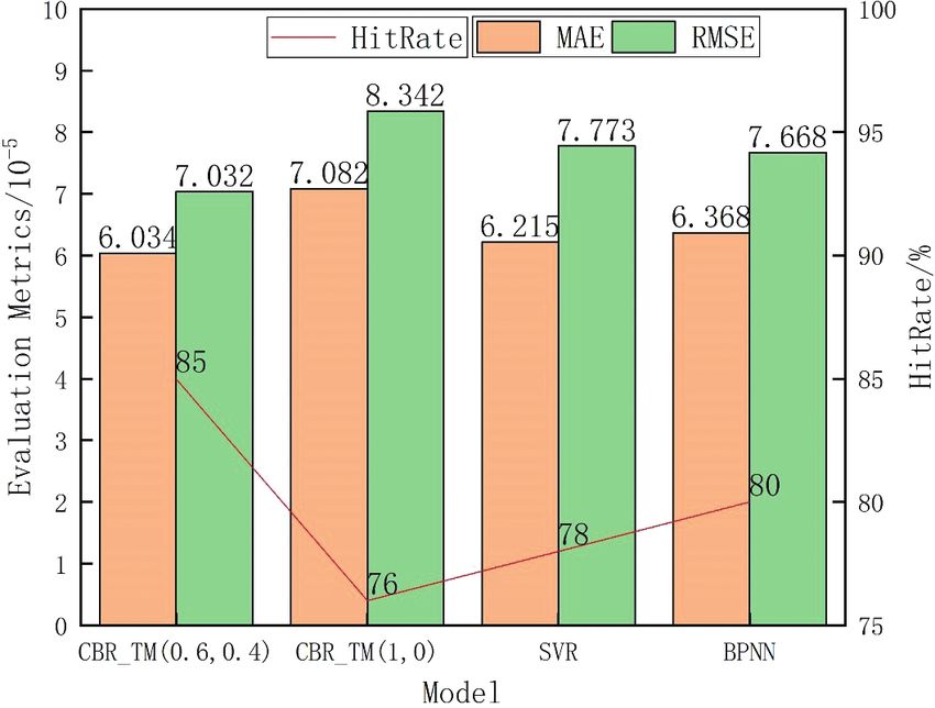
ISIJ International, Advance Publication by J-STAGE
                                      ISIJ International,
                                            ISIJ International,
                                                          Advance
                                                                Vol. Publication
                                                                     61 (2021), No.
                                                                                 by J-Stage
                                                                                    10

steel temperature in LF refining,9) Han Min et al. established       of certain weight were added in different batches into the
an end-point prediction model for converter steelmaking              converter; and, oxygen blown into the converter reacts with
based on membrane algorithm evolving extreme learning                elements in hot metal, such as carbon, silicon, manganese
machine.10) Wang Xiaojun et al. proposed end-point tem-              and phosphorus, producing slag and furnace gas;
perature prediction models in LF refining are respectively              (3) Since about 80% of the total oxygen consumption
based on random forest and ensemble of regression trees              was blown into the metal pool, a sublance was lowered to
of bootstrap feature subsets.11,12) He Fei et al. established        measure carbon content and temperature (i.e., “TSC”) of hot
an end-point prediction model in LF based on CBR.13) An              metal within the molten pool and take samples for testing;
improved CBR model based on mechanism model similarity                  (4) According to “TSC” measurement results, oxygen
was proposed by Feng Kai et al. to predict endpoint phos-            volume and coolant addition were adjusted in the subse-
phorus content in dephosphorization converters.14) Wang              quent blowing process;
Xinzhe et al. proposed a CBR model based on causality for               (5) As the blowing stage was completed, the sublance was
static control of converter steelmaking.15) Jiang Shenglong          lowered again to measure carbon content and temperature
et al. proposed a hybrid model based on multiple linear              (i.e., “TSO”) of molten steel and depending on correspond-
regression and Gaussian process regression for predicting            ing measurement results, a decision of tapping or reblowing
oxygen consumption in converter.16) Yan Liangtao et al.              was made;
proposed a predicting model of carbon content at end point              (6) After the smelting, the converter was shaked to tap
based on kernel partial least squares regression of genetic          the molten steel into a ladle, and alloy was also added at
algorithm (GA-KPLSR) in converter steel-making.17) A                 the same time;
multi-task learning (MTL) data-driven endpoint prediction               (7) After the tapping, slag-splashing was performed to
approach was established by Cheng Jin et al. for steelmak-           protect of the converter lining in some cases; and the entire
ing.18) Lv Wu proposed a novel process modeling method               process may be completed after slag splashing.
for steel sulphur content soft sensing during ladle furnace
steel refining.19) Liang Yanrui et al. proposed a two-step           2.2. The Principles of Model
case-based reasoning method based on attributes reduction               CBR is a critical method in the field of artificial intel-
for predicting the endpoint phosphorus content.20) Wang              ligence. Once a new problem occurs, similar problems
Hongbing et al. proposed an integrated CBR model for                 that have been solved and corresponding solutions can be
predicting endpoint temperature of molten steel in AOD.21)           retrieved from the case library. By comparing differences in
Okura Toshinori proposed a high-performance prediction               backgrounds and time of occurrence of the present and the
of molten steel temperature in tundish through gray-box              previous problems, solutions to the latter may be adjusted
model.22) Ahmad Iftikhar et al. proposed a prediction model          and altered so that a modified solution can be used to settle
of molten steel temperature in steel making process with             the former.25) Procedures of CBR mainly consist of case
uncertainty by integrating gray-box model and bootstrap              description, case retrieval, case reuse, case revision and
filter.23)                                                           case retaining. Among them, case retrieval is a key link.
    Although the above prediction models can predict the             A flow chart of a CBR algorithm has been presented in
end-point of the processes in steelmaking process more               Fig. 2.26)
accurate than the mechanism models. However, the mod-
els didn’t fully consider the time-series type data such             2.2.1. Case Description
as oxygen lance position, oxygen flow and bottom blow                   Case description, also known as case representation, is
gas flow. These time-series type process parameters have             deemed as a basis for case based reasoning. It is aimed at
an important influence on the end-point composition                  describing a case in a certain way. Generally, case descrip-
and temperature in converter. To solve this problem, an              tion involves feature description and solution description
improved CBR model using time-series data in converter               for a case. As for converter endpoint influence factors, they
was proposed to predict the end-point carbon content and             are given in Fig. 3.
temperature in converter.                                               In accordance with influence factors on converter end-
    The remaining sections are organized as follows: estab-          point compositions and temperature, corresponding data can
lishment of the endpoint prediction model in converter is            be categorized into the following two types:
presented in Section 2, the experiments and discussions are             (1) Single-valued Data
presented in Section 3, and Section 4 contains conclusion.              Single-valued data primarily include information about
                                                                     hot metal (e.g., temperature, weight, carbon content, silicon
                                                                     content, manganese content, phosphorus content and sul-
2.   Establishment of the Endpoint Prediction Model in
                                                                     phur content), amount of scrap added, amount of auxiliary
     Converter
                                                                     raw materials added (e.g., lime, dolomite and sinter) and gas
2.1. The Procedures of Converter Steelmaking Process                 consumption (e.g., oxygen and argon).
   The main procedures of a conventional converter can be               (2) Time Series Data
described in Fig. 1.24)                                                 Here, time series data consist of oxygen flow, oxygen
   (1) In each converter process, a certain proportions of           lance position and bottom-blowing gas flow.
molten hot metal and scraps were loaded in a converter;                 Therefore, structure of a case can be described as that
   (2) Then the oxygen lance was lowered to blow the oxy-            shown in Fig. 4, that is, Case = {Single-valued dataset,
gen into a molten pool at a certain rate; at the same time,          time series dataset}, where single-valued dataset = {Hot
auxiliary raw materials (e.g., lime, dolomite and sinter)            metal information (e.g., compositions and temperature),

© 2021 ISIJ                                                      2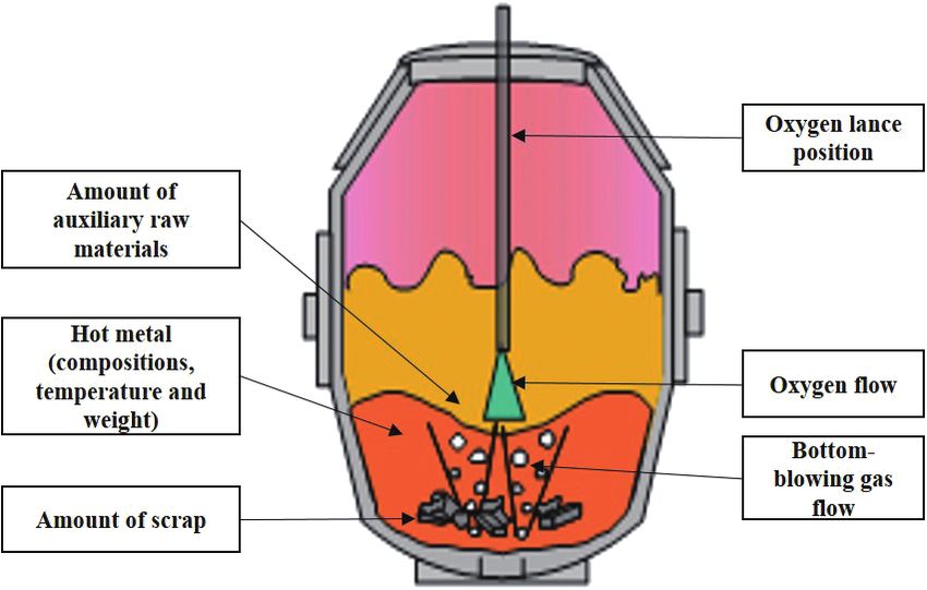
ISIJ International, Advance Publication by J-STAGE
                                       ISIJ International,
                                             ISIJ International,
                                                           Advance
                                                                 Vol. Publication
                                                                      61 (2021), No.
                                                                                  by J-Stage
                                                                                     10

                                              Fig. 1.   The main procedures of the converter.

                                                                                   Fig. 3.    The influence factors of end-point of converter.
               Fig. 2. The process of CBR model.

                                                   Fig. 4. The analysis of case attributes.

auxiliary raw materials (e.g., scrap, lime and dolomite), gas                Similarity of single-valued data can be calculated by
consumption (e.g., oxygen and argon)} and time series data-               various algorithms, such as the Euclidean distance and grey
set = { oxygen flow, oxygen lance height and argon flow}.                 distance. In this paper, the Euclidean distance is selected
                                                                          for similarity calculations. The Euclidean distance between
2.2.2. Case Retrieval                                                     the new case and a case in the case base can be expressed
   Case retrieval is to find the same or similar case in the              in Eq. (1).
case library according to case description of the case to be
solved. However, under circumstances that a case has many                                                      m

feature attributes, there is no identical cases in the case                                     d(X, Y)      w j [( x j  y j )2 ] .................... (1)
                                                                                                              j 1
library. So a certain calculation method are needed to find
the most similar case.                                                       Where, m is the number of influence factors on a case
   In consistency with description of case attributes, the                is; xj denotes the jth influencing factor of the new case; yj
similarity calculation methods for the single-valued type                 denotes the jth influencing factor of a case in a case library;
data and time-series type data were performed respectively.               wj is the weight of the jth influencing factor.
   (1) Single-valued Data Similarity                                         Similarity between the cases can be calculated by the

                                                                      3                                                                   © 2021 ISIJ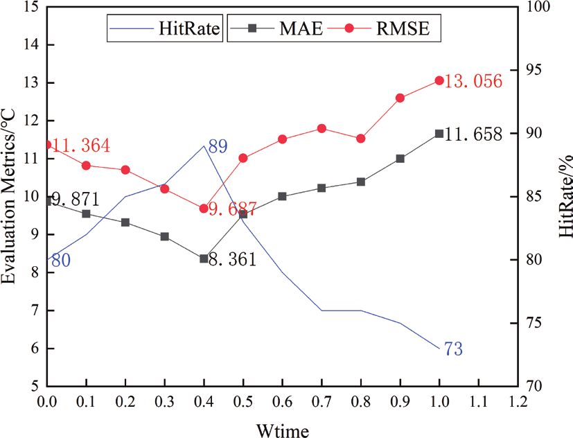
ISIJ International, Advance Publication by J-STAGE
ISIJ International,
ISIJ International,
Advance
Vol. Publication
61 (2021), No.
by J-Stage
10
following Eq. (2). (KNN) algorithm was selected to solve the problem, as
expressed in the following Eq. (7):
1
Gsim ( X ,Y ) ........................ (2)
1
d ( X ,Y )
Si
Ti ............................... (7)
k
T i 1k
(2) Time Series Data Similarity
Similarity of time-series data can be calculated by various
i 1Si
methods. Roughly, such similarity calculation methods are In the above equation, k denotes the number of reused
classified into two categories. One is trajectory point based cases, Si denotes the comprehensive similarity between the
similarity measurement; and, the other is the trajectory seg- new case and the ith most similar case, Ti denotes the solu-
ment based similarity calculation.27) As for the former, it tion of the ith most similar case.
consists of similarity calculation based on global and partial
matching respectively. More particularly, the global match-
3. Experiments and Discussions
ing based measurement approaches cover the Euclidean
distance model, Dynamic time warping (DTW) and Edit 3.1. Datasets
Distance on Real Penalty (ERP). Considering that time- To validate prediction accuracy of the proposed model,
series type data in the converter are featured with different 946 items of the actual production data from B steelworks
lengths, DTW is adopted here to calculate similarities of are used for such validation. Moreover, they are divided
this type data. Assumed two time series as A = {A1, A2, …, into a training set (including 846 items of data) and a test
Ai, …, AN} and B = {B1, B2, …, Bi, …, BM} were designed set (including 100 items of data). Depending on the field
firstly. By means of DTW, the time shaft was bent so as data, 16 influence factors are selected from them. To be
to acquire the minimum distance between above two time more concrete, these influence factors consist of 13 single-
series and determine optimal matching relations of points. value type and 3 time-series type. As for the former, they
In this case, a difference between Ai and Bj that match each cover temperature of hot metal, weight of hot metal, carbon
other represents the distance for this moment. content in hot metal, silicon content in hot metal, manga-
With the goal of defining an optimal matching relation, A nese content in hot metal, phosphorus content in hot metal,
and B are utilized to form a N × M DTW matrix d expressed amount of scraps, amount of the added lime, amount of
in the following Eq. (3): the added dolomite, amount of the added sinter, concur-
rent heating reagent, total gas consumption and total argon
d1,1 d1,M consumption. In terms of the latter, they are constituted by
d
......................... (3) oxygen flows, oxygen lance height and bottom-blowing
d N ,1 d N ,M argon flows. The time interval of time series data collection
is 5 seconds. The statistical results of influencing factors
In such a DTW matrix, Eq. (4) below was adopted for a data were shown in Tables 1 and 2.
distance from start point (1, 1) to end point (N, M) in line Where: TSO[C] and TSO[T] denote the measurement results
with basic thoughts of dynamic programming. of end-point carbon content and end-point temperature. The
length of time-series in Table 2. means the time interval
DN ,M d N ,M
min
DN 1,M , DN 1,M 1 , DN ,M 1
....... (4)
between the end point and the beginning point of time-
Where, DN,M refers to a locally-optimal cumulative dis- series data.
tance. It is obtained by adding up distances between the
current point and its previous point. 3.2. Evaluation Metrics
Define the time-series similarity between two time series In order to evaluate the prediction accuracy of the mod-
A = {A1, A2, …, Ai, …, AN} and B = {B1, B2, …, Bi, …, els, three indexes are used to evaluate, which are the mean
BM} as: absolute error (MAE), the root mean square error (RMSE)
and hit rate of end-point (HitRate). The calculation formula
1
Dsim ( A, B) ......................... (5) is as follows:
1
DN , M
1 n
(3) Comprehensive Similarity MAE
yˆi
yi ........................... (8)
n i 1
The single-valued data similarities and time series data
similarities were weighted to obtain the comprehensive
1 n
similarity between the cases. As for the corresponding cal- yˆ RMSE
( yi
yˆi )2 ....................... (9)
n i 1
culation formula, it is presented below:
1 n
Ssim wsingle * Gsim ( X ,Y )
wtime *
Dsim ( Ai , Bi ) .... (6)
n i 1 HitRate
the number of yi
yˆi
errorbound
100%
n
Where, n denotes the number of time series data vari- ......................................... (10)
ables; wsingle and wtime denote respectively the weight of the
single-value data similarity and time-series data similarity, Where: yi and ŷi denote the actual and prediction of end-
wsingle + wtime = 1, the value is determined by the experiment. point temperature in the ith case; n is the size of the cases;
errorbound denote error range, the error range of carbon
2.2.3. Case Reuse content and temperature prediction model is 0.02% and
Subsequent to case retrieval, the k-nearest neighbor 15°C respectively in this paper.
© 2021 ISIJ 4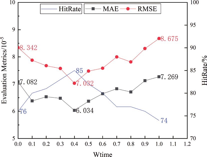
ISIJ International, Advance Publication by J-STAGE
                                                ISIJ International,
                                                      ISIJ International,
                                                                    Advance
                                                                          Vol. Publication
                                                                               61 (2021), No.
                                                                                           by J-Stage
                                                                                              10

                                             Table 1. Statistical results of influencing factors of single-value type.

                                  Influence factors                    Symbols     Mean.          Minimum              Maximum               Std.
                            temperature of hot metal/°C                   X1        1 437              1 080           1 264.22           120.40
                                Weight of hot metal/t                     X2          297              220                 275.53            10.55
                                       W[C]iron /%                        X3       4.6978             3.8001               4.2925         0.1442
                                       W[Si]iron /%                       X4      0.50622             0.00473          0.15441            0.09165
                                    W[Mn]iron /%                          X5      0.27224             0.00873          0.16096            0.02762
                                       W[P]iron /%                        X6      0.13164             0.04730              0.10261        0.01130
                                 Weight of Scrap/t                        X7          58.9             24.3                 45.22            4.453
                                 Amount of Lime/t                         X8       16.781              1.113               10.360            1.774
                               Amount of Dolomite/t                       X9       15.121              2.311                4.042            1.009
                                 Amount of Sinter/t                      X10       11.803               0                  2.6948         2.2516
                           Amount of heat supplementary/t                X11        4.078               0                  0.5964         0.82364
                             Oxygen consumption/Nm3                      X12       16 990             11 700               14 951            631
                                                                 3
                              Argon consumption/Nm                       X13          123               10                  40.77            34.29
                                           TSO[C]/%                       Y1       0.0443             0.01848              0.1281         0.01546
                                       TSO[T]/°C                          Y2        1 675              1 620                1 715            18.2

                                       Table 2.       Statistical results of the influencing factors of the time-series type.

       Influence factors       Mean              Maximum             Minimum     Maximum length of time-series                      Minimum length of time-series
                                   3                     3               3
         Oxygen flow       462/Nm /min 769/Nm /min 0/Nm /min                                     12/min                                            33/min
         lance position      1 411/mm            2 850/mm            1 197/mm                    13/min                                         34.5/min
                                       3                     3               3
          Argon flow         251/Nm /h           307/Nm /h           122/Nm /h                   13/min                                         34.5/min

3.3. Results and Analysis                                                                                   Table 3.       The weights of single-valued data.
   The parameters of the CBR_TM were set as follows: the                                                 X1           X2            X3        X4          X5          X6       X7
data standardization of single-valued type data adopts ( − 1,
                                                                                             Weight    0.0134     0.0119       0.0099 0.0641 0.0116 0.0082                    0.0578
1) standardization, the similarity calculation method was
based on Euclidean distance, the weight calculation method                                               X8           X9         X10         X11          X12         X13
is entropy weight method, and the number of reused case is                                   Weight    0.0162     0.0391       0.1653     0.4740         0.0111      0.1174
3. The weights of single-valued data was shown in Table 3.
   Dynamic warping (DTW) algorithm is used to calculate
the similarity of time-series data, and ( − 1, 1) standardiza-
                                                                                                             Table 4. The setting of ωtime in the model.
tion is also used for data standardization.
   wsingle and wtime were important parameters in the model,                                                    NO.           Symbols          wsin gle     wtime
the influence on the prediction accuracy was studied in this                                                      1         CBR_TM(1,0)            1           0
paper, the setting of wtime was shown in Table 4. The model
                                                                                                                  2        CBR_TM(0.9,0.1)         0.9         0.1
only consider the single-value data when wtime is 0 and only
consider the time-series data when wtime is 1.                                                                    3    CBR_TM(0.8,0.2)             0.8         0.2
   The statistics of prediction accuracy of the model with                                                        4        CBR_TM(0.7,0.3)         0.7         0.3
different wtime was shown in Figs. 5 and 6.                                                                       5    CBR_TM(0.6,0.4)             0.6         0.4
   It can be seen from the above figures that with the wtime
                                                                                                                  6    CBR_TM(0.5,0.5)             0.5         0.5
increases, the MAE and RMSE of models both show a trend
of first decreases and then increases and the HitRate of                                                          7    CBR_TM(0.4,0.6)             0.4         0.6
models show a trend of first increases and then decreases,                                                        8    CBR_TM(0.3,0.7)             0.3         0.7
It shows that the prediction accuracy of both carbon content                                                      9    CBR_TM(0.2,0.8)             0.2         0.8
and temperature prediction models first increases and then
                                                                                                                 10        CBR_TM(0.1,0.9)         0.1         0.9
decreases with the wtime increases. The model get the high-
est prediction accuracy when wtime was 0.4. For the carbon                                                       11         CBR_TM(0,1)            0           1
content prediction model, the MAE, RMSE and HitRate of
model with wtime = 0.4 were 6.034 × 10 − 5, 7.032 × 10 − 5, and
85%, respectively. Compared to the model with wtime =                                   For the temperature prediction model, the MAE, RMSE and
0, the MAE and RMSE were reduced by 1.048 × 10 − 5 and                                  HitRate of model with wtime = 0.4 were 8.361°C, 9.687°C,
1.310 × 10 − 5 respectively and HitRate increased by 9%.                                and 89%, respectively. Compared to the model with wtime =

                                                                                  5                                                                                   © 2021 ISIJ
ISIJ International, Advance Publication by J-STAGE
ISIJ International,
ISIJ International,
Advance
Vol. Publication
61 (2021), No.
by J-Stage
10
Fig. 5. Statistical results of evaluation metrics of carbon content Fig. 7. Comparison of evaluation metrics of different carbon con-
prediction models with different ω time. tent prediction models.
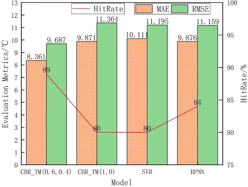
Fig. 6. Statistical results of evaluation metrics of temperature Fig. 8. Comparison of evaluation metrics of different temperature
prediction models with different ω time. prediction models.
0, the MAE and RMSE were reduced by 1.51°C and 1.68°C input layer node was 13, the number of first hidden layer
respectively and HitRate increased by 9%. nodes and the second layer nodes were 8 and 5 respectively.
Further analysis shows that the comprehensive utiliza- The number of output layer nodes was 1, the activation
tion of single-value type data and time series data in the function is ReLU. The comparison of the evaluation metrics
prediction model is helpful to improve the accuracy of results of different models was shown in Figs. 7 and 8.
the prediction model. However, the respective weights of It can be seen from the above figures that the performance
single-value type data and time-series type data should not of the CBR_TM(0.6,0.4) was better than the models based on
too high. Otherwise, the impact of a certain type on the CBR_TM(1,0), SVR and BPNN. The established model in
endpoint temperature is ignored, and the prediction accuracy this paper can meet the requirement of field production that
of the model is reduced. is the HitRate of the models more than 85%.
In order to further verify the accuracy of the model, the
prediction models based on support vector regression (SVR)
4. Conclusions
and Back Propagation Neural Network (BPNN) were also
established using the same single-value data in this paper. (1) An improved case-based reasoning model using
The SVR model was constructed by calling the SVR time-series data was established to predict the end-point
algorithm in the python data mining toolkit scikit-learn. The in the converter. The input variables of the model not only
parameters of the model was setting as follows, the polyno- includes single-value type data such as composition and
mial kernel (poly kernel) was selected as the kernel function temperature of hot metal but also includes the times-series
and the degree of the polynomial kernel function was three. type data such as lance position and oxygen flow, which
The BPNN model was constructed by calling the python makes the attributes of case more comprehensive. And the
deep learning toolkit tensorflow. The parameters of model similarity calculation method of time-series type data was
was setting as follows, the layers of network was four, the proposed based on dynamic time warping algorithm, which
© 2021 ISIJ 6ISIJ International, Advance Publication by J-STAGE
ISIJ International,
ISIJ International,
Advance
Vol. Publication
61 (2021), No.
by J-Stage
10
improves the accuracy of case retrieval.
REFERENCES
(2) The influence of the wtime on the prediction accu-
racy of the model was studied in this paper. The results 1) Y. Hu and L. He: Iron Steel Technol., 5 (2010), 7 (in Chinese).
2) W. Yan, C. Jiang and Z. Chen: 2019 Chinese Automation Cong.
show that the prediction accuracy of both carbon content (CAC), IEEE, New York, (2019), 43 (in Chinese).
and temperature prediction models first increases and then 3) C. Gao and M. Shen: Steelmaking, 35 (2019), No. 2, 20 (in Chinese).
4) C. Gao, M. Shen and X. Liu: Trans. Indian Inst. Met., 72 (2019), 257.
decreases with the wtime increases. The model get the high- 5) C. Gao, M. Shen and L. Wang: 37th Chinese Control Conf. (CCC),
est prediction accuracy when wtime was 0.4. For the carbon IEEE, New York, (2018), 3200.
content prediction model, the MAE, RMSE and HitRate of 6) M. Han and Y. Zhao: Expert Syst. Appl., 38 (2011), No. 12, 14786.
7) F. He and L. Zhang: J. Process Control, 66 (2018), 51.
model with wtime = 0.4 were 6.034 × 10 − 5 7.032 × 10 − 5, and 8) W. Lv, Z. Mao and M. Jia: 24th Chinese Control and Decision Conf.
85%, respectively. Compared to the model with wtime = (CCDC), IEEE, New York, (2012), 2362.
9) H. Tian and Z. Mao: IEEE Trans. Autom. Sci. Eng., 7 (2010), No. 1,
0, the MAE and RMSE were reduced by 1.048 × 10 − 5 and 73.
1.310 × 10 − 5 respectively and HitRate increased by 9%. 10) M. Han and C. Liu: Appl. Soft Comput., 19 (2014), 430.
11) X. Wang: IEEE/CAA J. Autom. Sin., 4 (2017), 770.
For the temperature prediction model, the MAE, RMSE and 12) X. Wang, M. You, Z. Mao and P. Yuan: Adv. Eng. Inform., 30
HitRate of model with wtime = 0.4 were 8.361°C, 9.687°C, (2016), No. 3, 368.
and 89%, respectively. Compared to the model with wtime = 13) F. He: Steel Res. Int., 11 (2018), 1079.
14) K. Feng, A. Xu, D. He and H. Wang: Steel Res. Int., 89 (2018), No.
0, the MAE and RMSE were reduced by 1.51°C and 1.68°C 6, 1800063.
respectively and HitRate increased by 9%. 15) X. Wang and M. Han: J. Dalian Univ. Technol., 51 (2011), No. 4,
593 (in Chinese).
(3) The prediction accuracy of established model 16) S. L. Jiang, X. Shen and Z. Zheng: Processes, 7 (2019), No. 6, 352.
(CBR_TM) is further compared with the models based on 17) L. Yan, M. Li and D. Yang: Control Eng. China, 24 (2017), No. 5,
SVR and BPNN. The MAE and RMSE of CBR_TM is lower 923 (in Chinese).
18) J. Cheng and J. Wang: J. Comput. Appl., 37 (2017), No. 3, 889 (in
than them and HitRate is higher than them, which proves the Chinese).
validity of the model. The CBR_TM can meet the require- 19) W. Lv: ISIJ Int., 59 (2019), 1276.
20) Y. Liang, H. Wang, A. Xu and N. Tian: ISIJ Int., 55 (2015), 1035.
ments of the field production. 21) H. Wang, A. Xu, L. Ai, N. Tian and X. Du: ISIJ Int., 52 (2012), 80.
22) T. Okura, I. Ahmad, M. Kano, S. Hasebe, H. Kitada and N. Murata:
Acknowledgement ISIJ Int., 53 (2013), 76.
23) I. Ahmad, M. Kano, S. Hasebe, H. Kitada and N. Murata: J. Chem.
This work is supported by the National Key Technol- Eng. Jpn., 47 (2014), 827.
ogy R&D Program of China (2017YFB0304000&2017 24) D. Sala, A. Jalalvand, A. Van Yperen-De Deyne and E. Mannens:
IEEE Int. Conf. on Machine Learning and Applications (ICMLA),
YFB0304001). IEEE, New York, (2018), 1419.
25) Y. Hou and C. Xu: J. Yanshan Univ. (Philos. Soc. Sci. Ed.), 12
(2011), No. 4, 108 (in Chinese).
26) X. Wang and J. Dong: Int. Conf. on Advanced Computational Intel-
ligence (ICACI), IEEE, New York, (2013), 130.
27) X. Zhou, G. Ji and S. Zhang: Geomat. World, 25 (2018), No. 4, 11
(in Chinese).
7 © 2021 ISIJYou can also read