A Novel Technique for Long-Term Anomaly Detection in the Cloud
←
→
Page content transcription
If your browser does not render page correctly, please read the page content below
A Novel Technique for Long-Term Anomaly Detection in the Cloud
                              Owen Vallis, Jordan Hochenbaum, Arun Kejariwal
                                                 Twitter Inc.

Abstract                                                                    z We build upon generalized Extreme Studen-
                                                                              tized Deviate test (ESD) [13, 14] and employ
High availability and performance of a web service is                         time series decomposition and robust statistics
key, amongst other factors, to the overall user experience                    for detecting anomalies.
(which in turn directly impacts the bottom-line). Exo-
                                                                            z We employ piecewise approximation of the
genic and/or endogenic factors often give rise to anoma-
                                                                              underlying long-term trend to minimize the
lies that make maintaining high availability and deliver-
                                                                              number of false positives.
ing high performance very challenging. Although there
exists a large body of prior research in anomaly detec-                     z We account for both intra-day and/or weekly
tion, existing techniques are not suitable for detecting                      seasonalities to minimize the number of false
long-term anomalies owing to a predominant underlying                         positives.
trend component in the time series data.                                The proposed technique can be used to automati-
   To this end, we developed a novel statistical tech-                  cally detect anomalies in time series data of both
nique to automatically detect long-term anomalies in                    application metrics such as Tweets Per Sec (TPS)
cloud data. Specifically, the technique employs statistical             and system metrics such as CPU utilization etc.
learning to detect anomalies in both application as well              r Second, we present a detailed evaluation of the pro-
as system metrics. Further, the technique uses robust sta-              posed technique using production data. Specifi-
tistical metrics, viz., median, and median absolute de-                 cally, the efficacy with respect to detecting anoma-
viation (MAD), and piecewise approximation of the un-                   lies and the run-time performance is presented.
derlying long-term trend to accurately detect anomalies
                                                                         Given the velocity, volume, and real-time nature of
even in the presence of intra-day and/or weekly season-
                                                                         cloud data, it is not practical to obtain time series
ality. We demonstrate the efficacy of the proposed tech-
                                                                         data with “true” anomalies labeled. To address this
nique using production data and report Precision, Recall,
                                                                         limitation, we injected anomalies in a randomized
and F-measure measure. Multiple teams at Twitter are
                                                                         fashion. We evaluated the efficacy of the proposed
currently using the proposed technique on a daily basis.
                                                                         techniques with respect to detection of the injected
1     Introduction                                                       anomalies.
Cloud computing is increasingly becoming ubiquitous.              The remainder of the paper is organized as follows: Sec-
In a recent report, IHS projected that, by 2017, enter-           tion 2 presents a brief background. Section 3 details the
prise spending on the cloud will amount to a projected            proposed technique for detecting anomalies in long-term
$235.1 billion, triple the $78.2 billion in 2011 [3]. In          cloud data. Section 4 presents an evaluation of the pro-
order to maximally leverage the cloud, high availability          posed technique. Lastly, conclusions and future work are
and performance are of utmost importance. To this end,            presented in Section 5.
startups such as Netuitive [1] and Stackdriver [2] have           2     Background
sprung up recently to facilitate cloud infrastructure mon-
                                                                  In this section, we present a brief background for com-
itoring and analytics. At Twitter, one of the problems we
                                                                  pleteness and for better understanding of the rest of the
face is how to automatically detect long-term anomalies
                                                                  paper. Let xt denote the observation at time t, where
in the cloud. Although there exists a large body of prior
                                                                  t = 0, 1, 2, . . ., and let X denote the set of all the obser-
research in anomaly detection, we learned, based on ex-
                                                                  vations constituting the time series. Time series decom-
periments using production data, that existing techniques
                                                                  position is a technique that decomposes a time series (X)
are not suitable for detecting long-term anomalies owing
                                                                  into three components, e.g., seasonal (SX ), trend (TX ),
to a predominant underlying trend component in the time
                                                                  and residual (RX ). The seasonal component describes the
series data. To this end, we propose a novel technique for
                                                                  periodic variation of the time series, whereas the trend
the same.
                                                                  component describes the “secular variation” of the time
The main contributions of the paper are as follows:
                                                                  series, i.e., the long-term non-periodic variation. The
    r First, we propose a novel statistical learning based        residual component is defined as the remainder of the
      technique to detect anomalies in long-term cloud            time series once the seasonality and trend have been re-
      data. In particular,                                        moved, or formally, RX = X - SX - TX . In the case of

                                                              1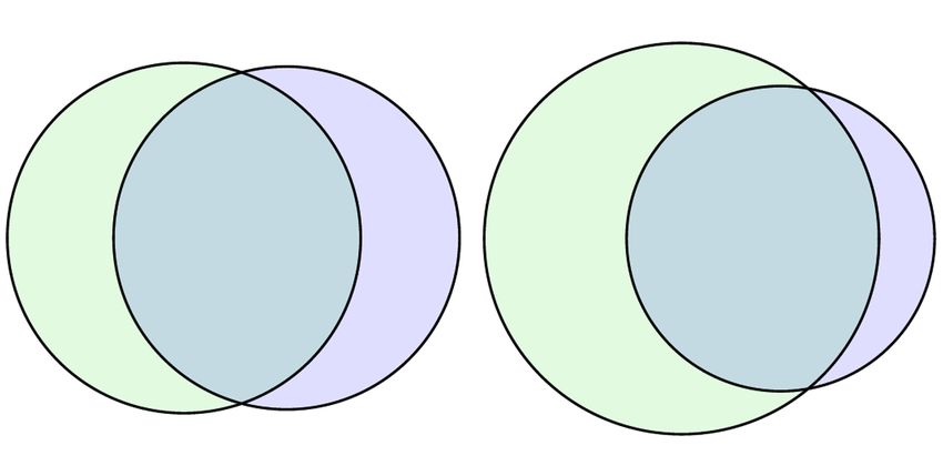
Raw                         Trend                             Adjusted Seasonal             Residual

                                                    (a) STL with Trend Removal
               Raw                         Median                            Adjusted Seasonal             Residual

                                                    (b) STL with Median Removal

                                Figure 1: STL (a) vs. STL Variant (b) Decomposition
long-term anomaly detection, one must take care in de-                 Time series decomposition facilitates filtering the
termining the trend component; otherwise, the trend may             trend from the raw data. However, deriving the trend,
introduce artificial anomalies into the time series. We             using either the Classical [15] or STL [4] time series de-
discuss this issue in detail in Section 3.                          composition algorithms, is highly susceptible to presence
   It is well known that the sample mean x̄ and standard            of anomalies in the input data and most likely introduce
deviation (elemental in anomaly detection tests such as             artificial anomalies in the residual component after de-
ESD) are inherently sensitive to presence of anomalies              composition – this is illustrated by the negative anomaly
in the input data [10, 9]. The distortion of the sample             in the residual, highlighted by red box, in Figure 1 (a).
mean increases as xt → ±∞. The proposed technique                   Replacing the decomposed trend component with the
uses robust statistics, such as the median, which is ro-            median of the raw time series data mitigates the above.
bust against such anomalies (the sample median can tol-             This eliminates the introduction of phantom anomalies
erate up to 50% of the data being anomalous [7, 6]).                mentioned above, as illustrated by the green box in Fig-
In addition, the proposed technique uses median abso-               ure 1 (b). While the use of the median as a trend substi-
lute deviation (MAD), as opposed to standard deviation,             tution works well where the observed trend component
as it too is robust in the presence anomalies in the in-            is relatively flat, we learned from our experiments that
put data [8, 10]. MAD is defined as the median of the               the above performs poorly in the case of long-term time
absolute deviations from the sample median. Formally,               series wherein the underlying trend is very pronounced.
MAD = mediani ( Xi − median j (X j ) ).                             To this end, we explored two alternative approaches to
                                                                    extract the trend component of a long-term time series
3     Proposed Technique                                            – (1) STL Trend; (2) Quantile Regression. Neither of
This section details the novel statistical learning-based           the above two served the purpose in the current context.
technique to detect anomalies in long-term data in the              Thus, we developed a novel technique, called Piecewise
cloud. The proposed technique is integrated in the Chif-            Median, for the same. The following subsections walk
fchaff framework [12, 11] and is currently used by a                the reader through our experience with using STL Trend,
large number of teams at Twitter to automatically detect            Quantile Regression, and detail Piecewise Median.
anomalies in time series data of both application metrics
such as Tweets Per Sec (TPS), and system metrics such               3.2       STL Trend
as CPU utilization.                                                 STL [4] removes an estimated trend component from the
   Twitter data exhibits both seasonality and an underly-           time series, and then splits the data into sub-cycle series
ing trend that adversely affect, in the form of false pos-          defined as:
itives, the efficacy of anomaly detection. In the rest of
                                                                    Definition 1 A sub-cycle series comprises of values at
this section, we walk the reader through how we mitigate
                                                                    each position of a seasonal cycle. For example, if the se-
the above.
                                                                    ries is monthly with a yearly periodicity, then the first
3.1    Underlying Trend                                             sub-cycle series comprised of the January values, the
                                                                    second sub-cycle series comprised of the February val-
In Twitter production data, we observed that the underly-
                                                                    ues, and so forth.
ing trend often becomes prominent if the time span of a
time series is greater than two weeks. In such cases, the              LOESS smooths each sub-cycle series [5] in order to
trend induces a change in mean from one (daily/weekly)              derive the seasonality. This use of sub-cycle series allows
cycle to another. This limits holistic detection of anoma-          the decomposition to fit more complex functions than the
lies in long-term time series.                                      classical additive or the multiplicative approaches. The

                                                                2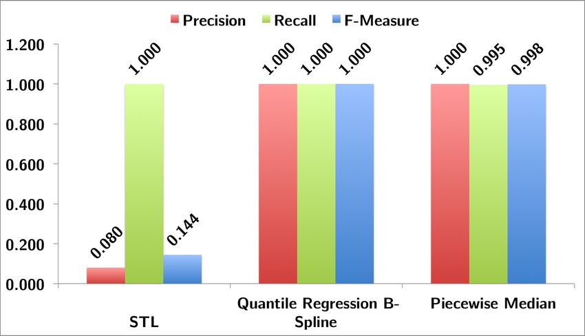
Figure 2: An illustration of the trends obtained using different approaches
estimated seasonal component is then subtracted from enough data points to decompose the seasonality, while
the original time series data; the remaining difference is also acting as a usable baseline from which to test for
smoothed using LOESS, resulting in the estimated trend anomalies. The red line in Figure 2 exemplifies the trend
component. STL repeats this process, using the most re- obtained using the piecewise approach.
cent estimated trend, until it converges on the decompo- We now present a formal description the proposed
sition, or until the difference in iterations is smaller then technique. Algorithm 1 has two inputs: the time series
some specified threshold. The purple line in Figure 2 X and maximum number of anomalies k.
exemplifies the trend obtained using STL for a data set
obtained from production. Algorithm 1 Piecewise Median Anomaly Detection
1. Determine periodicity/seasonality
3.3 Quantile Regression
2. Split X into non-overlapping windows WX (t) con-
While least squares regression attempts to fit the mean
taining at least 2 weeks
of the response variable, quantile regression attempts to
fit the median or other quantiles. This provides statisti-
cal robustness against the presence of anomalies in the for all WX (t) do
data. Marrying this with a B-spline proved to be an ef- Require:
fective method for estimating non-linear trends in Twit- nW = number of observations in WX (t)
ter production data that are longer then two weeks. This k ≤ (nW × .49)
extracts the underlying trend well for long-term time se- 3. Extract seasonal SX component using STL
ries data. However, we observed that it would overfit the
4. Compute median X̃
trend once the data was two weeks or less in length. This
meant that large blocks of anomalies would distort the 5. Compute residual RX = X − SX − X̃
spline and yield a large number of both False Negatives /* Run ESD / detect anomalies vector XA with X̃ and
(FN) and False Positives (FP). The aforementioned pit- MAD in the calculation of the test statistic */
fall (meaning, overfitting) on two-week windows means 6. XA = ESD(RX , k)
that Quantile B-spline is not applicable in a piecewise 7. v = v + XA
manner, and as such, provided further motivation for a end for
piecewise median approach. Additionally, from the fig- return v
ure we note that Quantile Linear, the line in green, also
poorly fits the long-term trend. It is important to note that the length of the windows in
the piecewise approach should be chosen such that the
3.4 Piecewise Median windows encompasses at least 2 periods of any larger
In order to alleviate the limitations mentioned in previ- seasonality (e.g., weekly seasonality owing to, for exam-
ous subsections, we propose to approximate the under- ple, weekend effects). This is discussed further in Sec-
lying trend in a long-term time series using a piecewise tion 4.1
method. Specifically, the trend computed as a piecewise
combination of short-term medians. Based on experi- 4 Evaluation
mentation using production data, we observed that sta- The use of different trend approximations yields different
ble metrics typically exhibit little change in the median sets of long-term anomalies. First, we compare the effi-
over 2 week windows. These two week medians provide cacy of the proposed Piecewise Median approach with
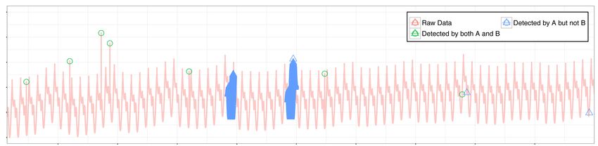
3Figure 3: Anomalies found using STL (top), Quantile B-spline (middle), and Piecewise Median (bottom)
Figure 5: Intersection and Difference between anomalies detected using two-week piecewise windows containing
partial weekend periods (A) and full weekend periods (B)
STL and Quantile Regression B-Spline. Second, we re- aggressive towards the end of the time series, yielding
port the run-time performance of each. Lastly, we com- many false positives. In contrast, Piecewise Median de-
pare how the proposed technique fared against ground tects the majority of the intra-day anomalies, and has
truth (via anomaly injection). a much lower false positive rate than STL. These in-
sights also mirror Figure 4, wherein we note that roughly
4.1 Efficacy 45% of the anomalies found by Piecewise Median are the
We evaluated the efficacy of the proposed Piecewise Me- same as STL and B-spline, with B-spline being the more
dian approach using production data. In the absence of conservative.
classification labels, i.e., whether a data point is anoma-
lous or not, we worked closely with the service teams PIECEWISE STL PIECEWISE QUANTILEB- SPLINE
MEDIAN TREND MEDIAN REGRESSION
at Twitter to assess false positives and false negatives.
Figure 3 exemplifies how STL, Quantile Regression B-
Spline, and Piecewise Median fare in the context of
anomaly detection in quarterly data. The solid blue lines 28.
47 46.
15 25.
37 45.
33 44.
46 10.
21
show the underlying trend derived by each approach.
From the figure, we note that all the three methods are
able to detect the most egregious anomalies; however,
we observe that the overall anomaly sets detected by
the three techniques are very different. Based on our Figure 4: Intersection and set difference of anomalies
conversation with the corresponding service teams, we found in STL and Quantile B-spline vs. Piecewise Me-
learned that STL and Quantile Regression B-Spline yield dian
many false positives. The Quantile Regression B-Spline In production data, we observed that there might be
appears to be more conservative, but misses anomalies multiple seasonal components at play, for example daily
in the intra-day troughs. By comparison, STL detects and weekly (e.g., increased weekend usage). In light of
some of these intra-day anomalies, but it becomes overly this, the Piecewise Median assumes that each window
4captures at least one period of each seasonal pattern. The
implication of this is illustrated in Figure 5 which shows
intersection and differences between the set of anomalies
obtained using the Piecewise Median approach using the
same data set but “phase-shifted” to contain partial (set
A) and full (set B) weekend periods. From the figure we
note that anomalies detected using set A contains all the
anomalies detected using set B; however, the former had
a high percentage of false positives owing to the fact that
set A contained only the partial weekend period.
4.2 Run-time Performance
Figure 6: Precision, Recall, and F-Measure
Real-time detection of anomalies is key to minimize im-
pact on user experience. To this end, we evaluated the run-time of Piecewise Median analyzes larger time series
runtime performance of the three techniques. Piece- in a shorter period. This might prove useful where the
wise Median took roughly four minutes to analyze three detection of anomalies in historical production data can
months of minutely production data, while STL and provide insight into a time sensitive issue. Additionally,
Quantile B-spline took over thirteen minutes. Table 1 from Figure 6 we note that Piecewise Median performs
summarizes the slowdown factors. From the table we almost as well as Quantile B-spline, while STL has very
note a slow down of > 3× which becomes prohibitive low precision.
when analyzing annual data. From the results presented in this section, it is evi-
dent that Piecewise Median is a robust way (has high
Avg Percentage F-measure) for detecting anomalies in long term cloud
Slowdown
Minutes Anomalies data. Further, Piecewise Median is > 4× faster!
STL Trend 13.48 3.19x 8.6% 5 Conclusion
Quantile B-Spline 13.62 3.22x 5.7% We proposed a novel approach, which builds on ESD, for
Piecewise Median 4.23 1x 9.5% the detection of anomalies in long-term time series data.
This approach requires the detection of the trend compo-
Table 1: Run time performance
nent, with this paper presenting three different methods.
4.3 Injection based analysis Using production data, we reported Precision, Recall,
Given the velocity, volume, and real-time nature of cloud and F-measure, and demonstrated the efficacy of using
infrastructure data, it is not practical to obtain time series Piecewise Median versus STL, and Quantile Regression
data with the “true” anomalies labeled. Consequently, B-Spline. Additionally, we reported a significantly faster
we employed an injection-based approach to assess the run-time for the piecewise approach. In both instances
efficacy of the proposed technique in a supervised fash- (efficacy and run-time performance), the anomaly detec-
ion. We first smoothed production data using time series tion resulting from Piecewise Median trend performs as
decomposition, resulting in a filtered approximation of well, or better then, STL and Quantile Regression B-
the time series. Anomaly injection was then randomized Spline. The technique is currently used on a daily ba-
along two dimensions – time of injection, and magnitude sis. As future work, we plan to use the proposed ap-
of the anomaly. Each injected data set was used to create proach to mitigate the affect of mean shifts in time series
nine different test sets (time series), with 30, 40, and 50% on anomaly detection.
of the days in the time series injected with an anomaly at References
1.5, 3, and 4.5σ (standard deviation). The 1σ value was [1] Netuitive. http://www.netuitive.com.
derived from the smoothed times series data. [2] Stackdriver. http://www.stackdriver.com/.
[3] Cloud- related spending by businesses to triple from 2011 to 2017, Feb.
As with the actual production data, STL and Quantile 2014.
[4] C LEVELAND , R. B., C LEVELAND , W. S., M C R AE , J. E., AND T ERPEN -
B-Spline exhibit a 4× slowdown (see Table 2). The faster NING , I. STL: a seasonal-trend decomposition procedure based on loess.
Journal of Official Statistics 6, 1 (1990), 373.
[5] C LEVELAND , W. S. Robust locally weighted regression and smoothing
Avg Minutes Slowdown scatterplots. Journal of the American statistical association 74, 368 (1979),
829–836.
[6] D ONOHO , D. L., AND H UBER , P. J. The notion of breakdown point. A
STL Trend 21.59 4.49x Festschrift for Erich L. Lehmann (1983), 157184.
Quantile B-Spline 21.48 4.78x [7] H AMPEL , F. R. Contributions to the theory of robust estimation. University
of California, 1968.
Piecewise Median 4.49 1x [8] H AMPEL , F. R. The influence curve and its role in robust estimation. Jour-
nal of the American Statistical Association 69, 346 (1974), 383–393.
[9] H AMPEL , F. R., RONCHETTI , E., ROUSSEEUW, P. J., AND S TAHEL ,
Table 2: Run time performance in case of anomaly injec- W. A. Robust statistics: the approach based on influence functions. Wiley,
New York, 1986.
tion
5[10] H UBER , P. J., AND RONCHETTI , E. Robust statistics. Wiley, Hoboken,
N.J., 1981.
[11] K EJARIWAL , A., L EE , W., VALLIS , O., H OCHENBAUM , J., AND YAN , B.
Visual analytics framework for cloud infrastructure data. In Computational
Science and Engineering (CSE), 2013 IEEE 16th International Conference
on (Dec 2013), pp. 886–893.
[12] L EE , W., K EJARIWAL , A., AND YAN , B. Chiffchaff: Observability and
analytics to achieve high availability. In Large-Scale Data Analysis and
Visualization (LDAV), 2013 IEEE Symposium on (Oct 2013), pp. 119–120.
[13] ROSNER , B. On the detection of many outliers. Technometrics 17, 2
(1975), 221227.
[14] ROSNER , B. Percentage points for a generalized ESD many-outlier proce-
dure. Technometrics 25, 2 (1983), 165172.
[15] S TUART, A., K ENDALL , M., AND O RD , J. K. The advanced theory of
statistics. Vol. 3: Design and analysis and time-series. Griffin, 1983.
6You can also read