A new look into Off-ball Scoring Opportunity: taking into account the continuous nature of the game - FC Barcelona ...
←
→
Page content transcription
If your browser does not render page correctly, please read the page content below
A new look into Off-ball Scoring Opportunity:
        taking into account the continuous nature of the game
                    Hugo M. R. Rios-Neto, Wagner Meira Jr., Pedro O. S. Vaz-de-Melo

                                 Universidade Federal de Minas Gerais, Brazil
                                {hugoriosneto, meira, olmo}@dcc.ufmg.br

     Abstract
  With the rise of tracking data, sports analytics can influence the game’s tactical aspects like never
before. In football, measuring the quality of the players’ positioning to receive a pass in condition
to score has much value. The Off-Ball Scoring Opportunity model was built to do just that. With
that, players receive credit for being well-positioned to score, even if a teammate cannot get them
the ball. It was originally modeled to consider the game’s snapshot only when a player executes an
action. However, football is a continuous sport, where decision-making happens at all times, and
actions are not discretized as in sports such as baseball and American football. In this paper, we
propose a reinterpretation of the original model, where the Off-Ball Scoring Opportunity is calculated
for every timestep an attacking player has the ball at his feet. It makes sense, since as long as a
player has control of the ball, he can move it somewhere else on the pitch. Through this new form of
applying the Off-Ball Scoring Opportunity model, we can build time-series that represent the scoring
probability of the next on-ball event at any given moment in time. Later, we demonstrate how this
way of using the model offers a much more in-depth view of attacking creation at an individual and
team level.
     Keywords
     data mining, spatiotemporal analysis, sports analytics, football

1.    INTRODUCTION

Tracking data has allowed for much deeper comprehension and analysis of football, making it possible
to evaluate not only what happens around the ball but the game as a whole. One of the biggest
challenges is to create ways of analyzing the game quantitatively that is logical to the decision-making
process that is intrinsic to the game. In some way, models should incorporate the thought-process
behind an ideal action at a collective or individual level.
  In that sense, a model called Off-Ball Scoring Opportunity (OBSO) [Spearman 2018] was developed
to evaluate players’ off-ball positioning that could lead to goals. Spearman’s work’s main objective
was to create a metric that is a better predictor of future goals than past goals or shots by rewarding
players for good positioning in areas where they can receive a pass, control the ball, and score. The
model is very intuitive since its steps are answers to football-specific questions, such as "where will
2 · the ball move to?" and "which areas on the field are controlled by each team?". However, this model uses tracking data only from the timestamps of the game that match event data. With that, we can only analyze the off-ball positioning of attackers when the action was executed. For example, suppose a player dribbles the ball for a long time and decides to pass the ball at some point. In that case, we will only have information about the passing possibilities at the time the player passed the ball. If better passing opportunities were available earlier in that player’s run, the model would not capture that. It makes sense to view the OBSO model as a continuous time-series because, as a player, you do not know when your teammate will pass you the ball, so the amount of time you make yourself available to receive that pass is relevant. In this paper, we propose a new way of using the Off-Ball Scoring Opportunity model, where a player can transition the ball to himself (not only passes) and all on-ball touches are relevant instead of only on-ball events. We apply our methodology to a small public dataset containing some goals Liverpool scored during 2019. Later, we present three primary forms of evaluating attacking plays using our methods. Finally, we discuss some practical applications of our work and how this different approach may fit Football better due to its continuous nature. 2. DATA In this work, we analyze broadcast tracking data from 18 out of 19 goals Liverpool scored during 2019 that are present in a public dataset [Tavares 2020]. All the goals utilized in this article were scored from open play, which means they were not following set-pieces (corners, free-kicks, and penalties). The goal in the dataset that was not used came from a corner and, for that reason, it would not serve the purpose of this work. The data was made available through the Friends of Tracking initiative. More information about the goals in the dataset are in Table 1. The data was collected using homography on video frames to extract the coordinates on the field for every player on the screen and the ball. Importantly, not every player is included in each play, even though all the players close to the ball are. The data was recorded at a frequency of 1-2Hz. Interpolation was made to turn it into 20Hz. This entire process was done by the creator of the dataset. Although the data lacks accuracy, since it was not originally collected for research purposes, it can still be beneficial for application purposes, due to the fact that spatiotemporal tracking data availability is very limited. Besides players’ positions, their velocities at every point in time are also crucial for applying the Off-ball Scoring Opportunity model. First of all, we calculate the displacement of every player and divided it by the timestep between frames (0.05 seconds). Secondly, we apply a moving average filter to smooth the velocities. We also set a maximum speed that a player can realistically reach, so that potential errors in the players’ positions do not yield enormous velocities that are unrealistic. 3. METHODS In this section, we will initial go through the Off-ball Scoring Opportunity (OBSO) model, pointing implementation differences from the original work, which were mostly due to lack of data, data in- naccuracies and for simplification purposes. Later, we will propose a different way of choosing the sequence of moments in which to calculate the OBSO, instead of only at the timestamp an event happens. 3.1 Off-ball Scoring Opportunity The OBSO model calculates the probability of the attacking team scoring after the next event, at a specific instant. For that to happen, the ball must move from where it is to somewhere else on the pitch, a player from the attacking team must control the ball, and such player must score after a shot.
·    3

                                           Goal                      Date       Time (s)
                             Liverpool [3] - 0 Bournemouth        09/02/2019      7.45
                                 Bayern 0 - [1] Liverpool         13/03/2019      8.25
                                Fulham 0 - [1] Liverpool          17/03/2019      9.15
                             Southampton 1 - [2] Liverpool        05/04/2019      12.85
                                  Liverpool [2] - 0 Porto         09/04/2019      9.75
                                  Porto 0 - [2] Liverpool         17/04/2019      12.85
                                 Liverpool [1] - 0 Wolves         12/05/2019      7.85
                                Liverpool [4] - 0 Norwich         09/08/2019      7.45
                                Liverpool [2] - 1 Chelsea         14/08/2019      9.75
                               Liverpool [2] - 1 Newcastle        14/09/2019      8.55
                                Liverpool [2] - 0 Salzburg        02/10/2019      9.55
                                  Genk 0 - [3] Liverpool          23/10/2019      9.15
                            Liverpool [2] - 0 Manchester City     10/11/2019      8.35
                                Liverpool [1] - 0 Everton         04/12/2019      9.95
                                Liverpool [2] - 0 Everton         04/12/2019      14.35
                             Bournemouth 0 - [3] Liverpool        07/12/2019      8.55
                                Liverpool [1] - 0 Watford         14/12/2019      11.25
                                Leicester 0 - [3] Liverpool       26/12/2019      6.25

Table I: Table with details about the data used in this work. The "Goal" column indicates from which attacking
play, that resulted in a goal, the data represents. For example, the first row is from Liverpool’s third goal against
Bournemouth, the second is Liverpool’s first goal against Bayern. The column "Date" displays the date of the game in
dd/mm/yyyy format and "Time (s)" shows the duration of the attacking play that resulted in a goal, in seconds. The
number of tuples of data from each goal would be the duration times the frequency of the data.

For each of those conditions, we can find the probability of it happening. By multiplying them all, we
get the likelihood of all of them occurring. These three probabilities are described below.

(1) Transition: the probability of the ball being transitioned from its original location to an arbitrary
    point, r on the pitch. Represented as Tr .
(2) Control: the probability that the ball, at this arbitrary point r, will be controlled by the attacking
    team. Represented as Cr .
(3) Score: the probability of scoring from this arbitrary point r. Represented as Sr .

  Therefore, the total probability of scoring after one transition of the ball, at a specific moment, is
defined as:

                                                    X
                                       P (S|D) =          P (Sr ∩ Cr ∩ Tr |D)                                     (1)
                                                    r∈R

where D is the game state at a specific moment, and R is the set of all the points on the field. The
instantaneous game state includes the position and velocity of every player. The probability in (1)
can be decomposed into a series of conditional probabilities, forming the following equation:

                                         X
                            P (S|D) =          P (Sr |Cr , Tr , D)P (Cr |Tr , D)P (Tr |D)                         (2)
                                         r∈R

  The transition, control, and score models will be explained in the following sections.

  3.1.1 Control Model.
The Control Model, defined as Potential Pitch Control Field (PPCF) [Spearman 2018], tries to quantify
the probability of each player controlling the ball at every location on the field, given the ball has
4 ·
moved to that location, which is equivalent to P (Cr |Tr , D). The longer a player is within a small
distance of the ball without interference from an opponent, the higher the player’s probability of
controlling the ball correctly. We also did not assume the ball would arrive instantaneously at the
destination. Hence, we considered the ball would take some time to get to this location. Differently
than in the original work, we did not use aerodynamic drag of the ball to calculate the time it would
take for a pass to reach a particular location. Instead, the ball’s travel time was defined as the distance
to the target position from the current ball position divided by a set ball velocity. For this analysis,
we used an average ball speed of 15m/s [Shaw 2020]. The following differential equation is used to
calculate the probability of each player controlling the ball in some location r, at time t.
!
dP P CF →
(t, − P P CFk (t, r , T |s, λj ) fj (t, →
→
− −
X
r , T |s, λj ) = 1− r , T |s)λj (3)
dT
k
In Equation 3, fj (t, →
−
r , T |s) is the probability that player j, at time t, can reach r, in less than time
T . This expression can be written as:
" #−1
T −τexp (t→
−
r)
→
−
fj (t, r , T |s)λj = 1 + e
−π √
3s (4)
where τexp (t→−
r ) is the expected intercept time, found by calculating the time it takes for the player
of interest to reach →−
r from →−
rj (t) with a starting speed →
−
vj (t), constant acceleration a, and maximum
2
velocity v. Like Spearman, we used 7m/s and 5m/s for a and v, respectively.
The variable λj in Equation 3 is the control rate, representing the inverse of the mean time it would
take a player to make a controlled touch on the ball. The higher the control rate, the less time it
takes a player to control the ball. Just as in the original model, λj was set to 3.99. When a player is
off-sides, his control rate is equal to zero. A per-player probability for control is built when Equation
3 is integrated over T from 0 to ∞.
3.1.2 Transition Model.
The Transition Model measures the probability of the next touch on the ball happening at a specific
location →−r . It is the last term in Equation 2. Since the distribution of displacements between
subsequent ball events is normally distributed [Spearman 2018], players tend to attempt short passes
with a higher frequency. Also, because of the angular variance when passing, as a player tries a long
pass, its target location will have a higher variance.
In principle, players pass the ball to where they think one of their teammates will control it. Since
the PPCF model gives the probability of the ball being controlled by the attacking team if it goes
to a specific location on the field, it can be superimposed with the normal distribution in order to
construct a decision probability density field. This way, decision making is incorporated into the
transition model.
" #α
T (t, →
−
r |σ, α) = N (→
−
r ,→
− P P CFk (t, →
−
X
r b (t), σ) · r) (5)
k∈A
In Equation 5, σ is related to the mean distance between on-ball events, A is the set of all attacking
players, α is a weight parameter for the PPCF model, and N is a two-dimensional normal distribution.
As Spearman, we set σ to 23.9 and α to 1.04. Equation 3 is normalized to unity.· 5
Fig. 2: This figure validates the logistic regression that was done to build the scoring probability model.
3.1.3 Score Model.
The first term in Equation 2, P (Sr |Cr , Tr , D), describes the probability of scoring from a certain
location r, given the ball has moved there and has been controlled by the attacking team. For
simplication purposes, the game state, D, will not be considered. Like Spearman, we built a data-
driven model to determine the probability of scoring from a specific point on the field. However,
instead of only considering the probability of scoring as a function of distance, we also considered the
angle formed between the player and the goal posts.
We define the scoring model as the probability of scoring from a shot as a function of distance and
goal angle [Sumpter 2020]. Since both variables show a strong relationship with the conversion ratio,
we can try to predict the probability of scoring using them. Intuitively, the probability of scoring goes
down as the distance grows and goes up as the angle gets larger. To model that, we use non-headers
shot data from an entire Premier League season [Pappalardo et al. 2019]. By getting the coordinates
from every shot, we are able to calculate the goal angle and distance and pair it with the outcome of
the shot to fit the best curve that describes the data. In this case, we perform a logistic regression,
described by the equation below:
1
S(t, →
−
r |c0 , c1 , c2 ) = (6)
1+ e−(c0 +c1 ·θ+c2 ·d)
where θ is the angle, in radians, formed between lines going from the ball to each of the goalposts and
d is the distance, in meters, from where the shot was made to the center of the goal. c0 , c1 and c2 are
the values that maximize the log-likelihood function. Their respective values are 0.7895, −1.2594, and
0.1155. One limitation of this model is that it overestimates the probability of scoring from headers,
since the model is built on non-header shots and headers have a lower conversion rate than regular
shots. Figure 1 details the logistic regression.
3.1.4 Final Probability.
By following the previous sections, we are able to calculate the probability of each of the three
conditional probabilities in Equation 2, from a specific location r, at time t. Finally, equation below
describes the probability of scoring after the next on-ball action, from a target position r on the field,
at time t.6 ·
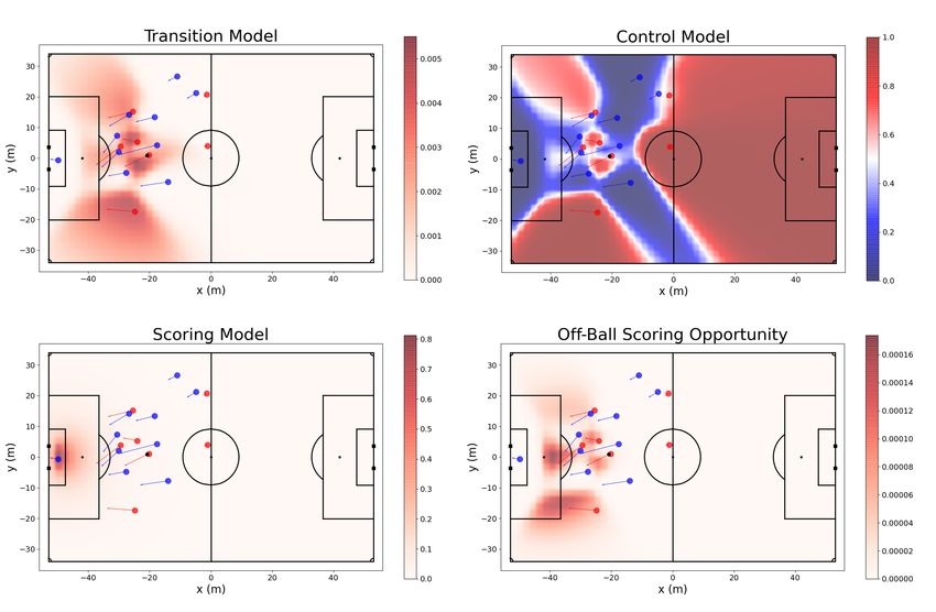
Fig. 3: This figure demonstrates each of the three intermediate steps and the combination of them all. The Transition
Model shows where the ball is most likely to go next. The Control Model shows which team would control the ball if it
moved there. The Scoring Model shows the likelyhood of scoring from a certain location. Finally, the Off-Ball Scorring
Opportunity model combines all of these probabilities. Cells are colored according to a colorbar that has the maximum
value in the grid as its darkest color. The red points are Liverpool players and blue points their opponent. The ball is
represented by the black point on the pitch.
OBSO(t, →
−
r ) = T (t, →
−
r ) · C(t, →
−
r ) · S(t, →
−
r) (7)
In Equation 7, T (t, →
−
r ) is the transition probability, C(t, →
−
r ) is the control probability and S(t, →
−
r)
is the scoring probability. To be able to visualize each of the intermediate probabilities, we calculate it
for every location on the field. For this analysis, the field was broken down into square cells, forming
a 32 × 50 matrix. Thus, for every cell, we calculate the conditional probabilities and multiply them
to get the final probability, for every point on the field. Figure 2 demonstrates that.
3.2 OBSO Space-Integration
At an instant t in time, by integrating through every point, r, on the field, we are able to get the total
probability of scoring after the next action on the ball. The OBSO space-integration, at a point in
time, is described by below. This is another form of writing Equation 1 and Equation 2.
32 X
50
OBSO(t, −
r→
X
OBSO(t) = ij ) (8)
i=1 j=1
In Equation 8, −
r→
ij is a tuple with the x and y coordinates of the field cell in the ith line and jth
column.· 7
Fig. 4: This figure shows the OBSO(t) function when each of the approaches is chosen. As we can see, the granularity
of the data by choosing the original approach (right) is significantly smaller. Also, the approach chosen for this work
(left) yields a time-series where OBSO(t) = 0 when the attack is not in control of the ball.
3.3 OBSO Time-Integration
In the original approach, Spearman considers the snapshot of the game only at the timestamp in
which the events happen. With that, we are able to capture the off-ball positioning of attacking
players independently of the completion of the event, meaning even if a player misses a square pass to
a striker inside the box, the striker’s positioning will be rewarded. However, football is a game where
decision-making is continuous and players can choose to move the ball to another location on the pitch,
as long as they are in control of the ball. By calculating the OBSO for every timestamp an atacking
player has control of the ball, we can have a deeper understanding of the attacking opportunity, both
in terms of collective space-creation and player decision-making. In this work, we manually tagged the
timestamps in which players had an on-ball touch and when the ball was not controlled by anyone (i.e.
the ball is being passed from one player to another). To our knowledge, data providers do not inform
about whether an attacking player was in control of the ball or not and that might be a limitation
to implementing this type analysis in a larger amount of data. Figure 2 demonstrates the difference
between the two different approaches.
After calculating the OBSO for every on-ball touch, we can perform an integration of those values
over time. The equation below describes integration over time, which is done the same way as in the
original work, but over more data points. The equation below describes how the time-integration.
N
X
OBSO = OBSO(t) (9)
t=1
In Equation 9, N is the number of timesteps of 0.05s and t is a variable that indicates tth timestep.
The obtained OBSO total is the cumulative sum of the OBSO value in every timestep. By doing
the integration on a larger amount of values, the OBSO metric loses its predictive property, as some
attacking opportunities yield values larger than 1, and thus does not represent the probability of the
play resulting in a goal. However, it is still a strong indicator of attacking quality, as plays with a high
integration value indicate that good transition options were offered for a larger amount of time. It
is intuitive to think that having certain transition options for a longer amount of time is better than
having a small time-window with the same alternatives, as only players with fast decision-making
might be able to take advantage of those short time-gaps of good transition opportunities that other
players will not.8 ·
OBSO
Goal max OBSO(t) OBSO n
Fulham 0 - [1] Liverpool 0.0919 2.851 0.0228
Liverpool [2] - 0 Porto 0.0284 1.272 0.0112
Leicester 0 - [3] Liverpool 0.0332 0.990 0.0215
Liverpool [2] - 0 Everton 0.0288 0.861 0.0049
Liverpool [1] - 0 Everton 0.0323 0.842 0.0073
Porto 0 - [2] Liverpool 0.0331 0.833 0.0066
Bayern 0 - [1] Liverpool 0.0206 0.804 0.0107
Liverpool [3] - 0 Bournemouth 0.0263 0.759 0.0099
Southampton 1 - [2] Liverpool 0.0205 0.684 0.0053
Liverpool [4] - 0 Norwich 0.0370 0.599 0.0098
Bournemouth 0 - [3] Liverpool 0.0372 0.492 0.0068
Liverpool [1] - 0 Watford 0.0149 0.429 0.0084
Liverpool [2] - 0 Salzburg 0.0341 0.403 0.0073
Genk 0 - [3] Liverpool 0.0215 0.266 0.0038
Liverpool [2] - 1 Chelsea 0.0186 0.255 0.0039
Liverpool [2] - 0 Manchester City 0.0309 0.209 0.0075
Liverpool [2] - 1 Newcastle 0.0295 0.197 0.0046
Liverpool [1] - 0 Wolves 0.0304 0.165 0.0127
Table II: Table with the values obtained by calculating each of the proposed metrics to every goal used from the dataset.
4. RESULTS
In this section, we will present the OBSO time-series for each of the goals used in from the dataset.
Also, we will evaluate those attacking opportunities using simple metrics derived from the OBSO
time-series and its integration. We focus on three different metrics to try!to have a better notion of
the quality of the attack: 1) max OBSO(1), OBSO(2), ..., OBSO(N ) , where N is the quantity
of 0.05s timesteps. 2) OBSO, time-integrated through the duration of the attack. 3) OBSO n , where
OBSO is calculated using Equation 9 and n is the number of timesteps in which the attacking team
had control of the ball, which is the entire time the ball is not in its trajectory of a pass or shot.
The first metric gives us the maximum value of the function OBSO(t). Therefore, by comparing
the maximum value for each of the goals, we can analyze how better one play was in comparison to
another, when the scoring chance was at its highest. The second metric gives us the time-integrated
OBSO(t) function as discussed in 3.3. It is also a good comparative measure because a play might
not have a maximum OBSO value that was high, but players might have had a much larger time on
the ball, in a slightly worse attacking chance. Finally, the third metric gives the mean OBSO value
for each goal, for the time an attacking player was in control of the ball. It can contribute to the
evaluation since an attacking play might not have a large integrated value due to the fact that the
ball stayed on the players’ feet for a short amount of time (i.e. one-touch passes were played), but the
scoring probability was high during those moments. Table 2 displays all the results, ordered by the
second proposed metric. Figures 4, 5 and 6 display the OBSO time-series for each of the goals.
5. PRACTICAL APPLICATIONS
Viewing attacking opportunities as OBSO time-series enables a more in-depth insight into how chances
are created through tracking data. Beyond identifying critical moments in a game and analysis of such
moments, player and team performance, and scouting, we believe this form of modeling can serve as a
tool for coaches when building their team’s attacking repertoire. For instance, low crosses across the
box have shown increased use by teams such as Liverpool and Manchester City. In those situations,
the main goal is for the attackers to create space where they can receive the ball and take a shot.
Also, since attackers do not know precisely when the ball will be played, they want to maximize the· 9 time-window where they can receive a pass. Independent of playing style, ultimately, teams should seek in the concluding stage of a possession: quality transition options, offered for the maximum amount of time, in a position where a teammate will control the ball and take a shot. Finally, we also believe the Control and Transition models should serve as the base for future research that tries to predict a near-future state of the game. The combination of these two models and a third one, which will give value to what we are trying to measure (in this case, scoring), can be used to model any phase of the game. REFERENCES Fernández, J. and Bornn, L. Wide Open Spaces: A statistical technique for measuring space creation in professional soccer. MIT Sloan Sports Analytics Conference, 2018. Pappalardo, L., Cintia, P., Ferragina, P., Massucco, E., Pedreschi, D., and Giannotti, F. PlayeRank: Data- driven Performance Evaluation and Player Ranking in Soccer via a Machine Learning Approach. ACM Transactions on Intelligent Systems and Technology 10 (5), 2019. Pappalardo, L., Cintia, P., Rossi, A., Massucco, E., Ferragina, P., Pedreschi, D., and Giannotti, F. A public data set of spatio-temporal match events in soccer competitions. Sci Data 6 (236), 2019. Shaw, L. Advanced football analytics: building and applying a pitch control model in python. https://www.youtube.com/watch?v=5X1cSehLg6st=18s, 2020. Spearman, W. Physics-Based Modeling of Pass Probabilities in Soccer. MIT Sloan Sports Analytics Conference, 2017. Spearman, W. Beyond Expected Goals. MIT Sloan Sports Analytics Conference, 2018. Sumpter, D. How to Build An Expected Goals Model 1: Data and Model. https://www.youtube.com/watch?v=bpjLyFyLlXs, 2020. Tavares, R. Last Row sample data. https://github.com/Friends-of-Tracking-Data-FoTD/Last-Row, 2020.
10     ·

Fig. 5: Time-series for the first eight goals used in this analysis (not ordered by our proposed evaluation). We can notice
different attacking patterns. Some plays showed an increase in OBSO through a long dribbling sequence (Southampton
1 - [2] Liverpool and Porto 0 - [2] Liverpool). Other goals saw an increase in value due to quick passing (Liverpool [1] -
0 Wolves).
·   11

Fig. 6: Time-series from goals in the dataset used in this analysis.
12    ·

                         Fig. 7: Time-series from goals in the dataset used in this analysis.

We would like to thank everyone involved with the Friends of Tracking initiative, a group of sports analytics experts
that took their time during the pandemic to teach newcomers about the state-of-the-art in soccer analytics. We would
also like to thank Gabin Rolland, who helped us implement and interpret the Off-Ball Scoring Opportunity model.
Finally, we would like to thank Ricardo Tavares for making the dataset available to the public. None of this work
would have been possible without all of you.
You can also read