Cluster-Based Statistical Arbitrage Strategy
←
→
Page content transcription
If your browser does not render page correctly, please read the page content below

Stanford University

                             MS&E 448

                 Big Data and Algorithmic Trading

Cluster-Based Statistical Arbitrage Strategy

   Authors:
   Anran Lu, Atharva Parulekar, Huanzhong Xu

                              June 10, 2018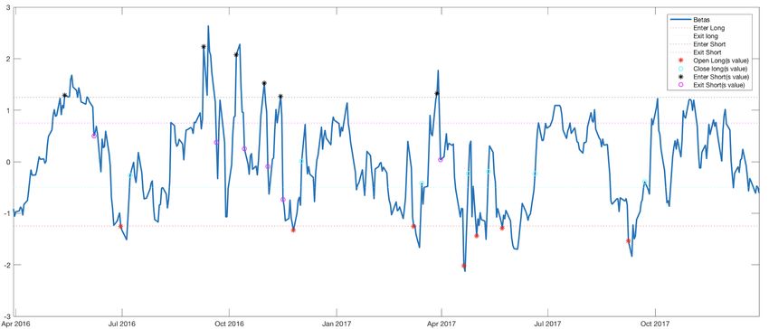
Cluster-Based Statistical Arbitrage Strategy

Contents
1. Introduction                                                                                                                                         2

2. Related Work                                                                                                                                         3

3. Data Preprocessing                                                                                                                                    4
   Quantopian . . . . . . . . . . . . . . . . . . . . . . . . . . . . . . . . . . . . . . . . . . . .                                                    4
   Yahoo Finance . . . . . . . . . . . . . . . . . . . . . . . . . . . . . . . . . . . . . . . . . .                                                     4

4. Classic Statistical Arbitrage                                                                                                                        4

5. Residual Prediction                                                                                                                                  5
   S-score Modelling Using AR-1 . . . . . . . . . . . . . . . . . . . . . . . . . . . . . . . . . .                                                     5
   Prediction Using LSTM . . . . . . . . . . . . . . . . . . . . . . . . . . . . . . . . . . . . .                                                      6

6. Stock Selection and Portfolio        Construction                                                                                                    7
   Alpha of Our Strategy . . . . . .    . . . . . . . . .   .   .   .   .   .   .   .   .   .   .   .   .   .   .   .   .   .   .   .   .   .   .   .   7
   Cointegration Test . . . . . . . .   . . . . . . . . .   .   .   .   .   .   .   .   .   .   .   .   .   .   .   .   .   .   .   .   .   .   .   .   7
   Clustering Method . . . . . . . .    . . . . . . . . .   .   .   .   .   .   .   .   .   .   .   .   .   .   .   .   .   .   .   .   .   .   .   .   8
   Portfolio Construction . . . . . .   . . . . . . . . .   .   .   .   .   .   .   .   .   .   .   .   .   .   .   .   .   .   .   .   .   .   .   .   9
   Trading Signal Generation . . . .    . . . . . . . . .   .   .   .   .   .   .   .   .   .   .   .   .   .   .   .   .   .   .   .   .   .   .   .   9

7. Simulation and Experiment Results                                                                   10
   Basic Modelling . . . . . . . . . . . . . . . . . . . . . . . . . . . . . . . . . . . . . . . . . . 10
   Experiments Results . . . . . . . . . . . . . . . . . . . . . . . . . . . . . . . . . . . . . . . 11

8. Conclusion and Further Discussion                                                                                                                    12

                                                                                                                                    Page 1 of 14
Cluster-Based Statistical Arbitrage Strategy
Abstract
In this paper, we study and develop the classical statistical arbitrage strategy developed by
Avellaneda and Lee [1]. Classical statistical arbitrage picks two highly correlated risky assets,
such as two stocks in a same sector, and generates trading signals when one of the stocks is
mispriced. For the first step we introduce an algorithm assigning each stock-ETF pair a score
based on the idea of cointegration test. Then we estimate for any given ETF which stocks we
should choose to perform pair tradings according to those scores. For the second step of the
classical strategy, we suggest how to apply LSTM to help us predict trading signals of a given
pair. Based on our simulation result, our model is valid for around first forty days in a trading
window considering the portfolio performance with its corresponding ETF.
1. Introduction
Statistical arbitrage is a financial strategy that employs pricing inefficiencies in mean-reverting
trading pairs of or buckets of securities. Classical statistical arbitrage strategy has systematic
trading signals, market-neutral trading book, considering zero beta, and statistical techniques to
generate positive returns.
One common statistical arbitrage strategy is pairs-trading. Pair usually consists of two risky
assets (such as two stocks) sharing similar characteristics, or in a same industry. For these kinds of
pairs, their returns are expected to track each other. In [1], they are described by the basic model
of pairs-trading:
dPt dQt
= αdt + β + dXt (1)
Pt Qt
where Pt and Qt are the corresponding price time series for stocks P and Q; α is negligible compared
to dXt ; β is determined by regression; and Xt is referred to as the cointegration residual. The basic
trading strategy is mainly determined by Xt . Generally, we long one dollar of stock P and short β
dollars of stock Q when Xt is small, or long β dollars of stock Q and short one dollar of stock P
when Xt is large.
In this paper, unless otherwise specified, a pair consists of a stock and an ETF. Figure 1
illustrates an example of how the stock price of Delta Airline, United Airline and the ETF of their
section, XLN, track each other, motivating us to choose a stock and an ETF as our mean-reverting
pair. Furthermore, in our trading strategy, we short a portfolio of weighted stocks and long the
ETF or long a portfolio of weighted stocks and short the ETF based on trading signals.
Since statistical arbitrage strategies do not perform well when the pair do not have two stocks
with prices tracking each other, we use cointegration scores to measure the correlation for a pair,
and select our buckets of stocks accordingly. To model mean-reversion, we use Ornstein-Uhlenbeck
(O-U) process to describe Xt :
dXt = κ(µ − Xt )dt + σdWt (2)
where κ is referred to as the mean reversion speed. The trading signal is computed by
Xt − EXt
s=
V arXt
Our statistical strategies are mostly based on clusters. Most related works so far cluster stocks
based on empirical returns or fundamental factors. However, previous cluster factors may cause
Page 2 of 14Cluster-Based Statistical Arbitrage Strategy
Figure 1: Stock chart of United Airline, Delta Airline and XTN
instability. In this paper, incorporated previous work, we have several innovations. First, instead
of clustering based on empirical returns, we choose mean-reversion time κ1 , residual st and coin-
tegration factors as our cluster factors. Second, we dynamically adjust pairs based on real time
factors. Third, we adopt a machine learning technique called Long Short Term Memory networks
(LSTMs) to help us make predictions.
In section 2, we talk about what related work has been done by other academic literature and
how we expand and innovate our work based on their research. In section 3, we discuss our data
set, including how we achieve data and how we deal with problems that we encounter when we
process our data. In section 4, we explain classic statistical arbitrage and how this becomes a
fundamental support to our research. In section 5, we mainly talk about two different approaches
we use to perform prediction of s-scores, including AR-1 and LSTM. In section 6, we include the
metrics and process of stock selection such as cointegration test, clustering method and portfolio
construction. In section 7, we test our model with some common simulation techniques. In section
8, we demonstrate our current results and discuss how our model performs. In section 9, we give a
conclusion to our entire research and how we might have some further improvement in the future.
2. Related Work
A lot of related work in statistical arbitrage has been done to inspire our idea in cluster-based
strategy. In [1], it gives a general overview for statistical arbitrage and equities market using the
idea of pairs-trading. It provides a traditional statistical arbitrage strategy and detailed algorithms
and equations, which allow people to expand their ideas based on [1]. However, it does not include
how we can include clustering to improve our portfolio selection. Inspired by [1]’s work, we perform
a statistical arbitrage strategy but incorporate clustering methods based on cointegration scores
and mean-reverting speed. [5] demonstrates how pairs-trading system is proposed with a two-stage
correlation and cointegration approach. It explains carefully on their cointegration process by
using ADF test adapted from Engle-Granger test. Different to [5]’s cointegration test, we use both
Engle-Granger test and Johansen’s test, which fit our model better. [2] mainly tests the validity
Page 3 of 14Cluster-Based Statistical Arbitrage Strategy
of cointegration in choosing stock pairs. It also estimates long-term equilibrium and model the
residuals. We apply similar ideas on cointegration test. However, since [2] selects Sao Paulo stock
exchanging as their universe, it does not apply to our universe S&P 500, which operates differently
from Sao Paolo stock.
3. Data Preprocessing
The main data we need for our project is historical stock and ETF prices. Note that since our
algorithm has a periodic cointegration test and trading experiment structure, we require the data
to be highly intact and consistent, i.e., it should offer a same reply for different requests asking for
a same piece of record.
Quantopian
Quantopian is a well-built online platform which offers a comprehensive dataset, a robust research
environment, and a close-to-reality backtest program. Unfortunately, there are two main reasons
this platform is not compatible with our project.
• Coding Language: Currently, the only language that Quantopian supports is Python. Some
key implementations of our trading strategy, for instance cointegration test functions, can not
be easily realized with Python packages. Therefore Matlab is necessary for the design of our
kernel.
• Stock Split: In the research environment, Quantopian does not deal with stock split ex-
plicitly. For a same stock which experienced stock split, requesting its price from different
but overlapping time periods may lead to different results. For instance, Apple stock prices
requested from January 2014 to June 2014 are not consistent with those requested from Jan-
uary 2014 to March 2014. Since for our strategy, repetitive requesting prices from a same
period happens frequently, we have to treat stock split in a different way than Quantopian
does.
Yahoo Finance
Yahoo Finance has a comprehensive record of historical stock prices, at least for S&P 500 stocks.
For any specific stock ticker, Yahoo Finance always offers consistent data and missing data is
explicitly labelled. Thus, we decide to fetch historical stock data from Yahoo Finance. Although
Yahoo Finance turned down its public API service during November 2017, it’s still possible to gain
data from its dataset via obtaining cookies and searching for crumb store. The data we obtain from
Yahoo are historical stock prices of all S&P 500 stocks from the past five years.
4. Classic Statistical Arbitrage
Statistical arbitrage exploits the mispricing between mean-reverting pairs of stocks or buckets of
stocks in a beta-neutral market. The term mean-reversion means the assumption that the stock
price tends to converge to the average price over time. Thus, the gap between the stock price and the
Page 4 of 14Cluster-Based Statistical Arbitrage Strategy
average price will close in the long run. Therefore, statistical arbitrage strategy makes profit from
this gap. For example, we can short a stock which has a price lower than expected because when
the gap narrows, we can make profit from this spread. In [1], it presents the statistical arbitrage
model about two stocks which tracks each other and thus, provides profitable opportunity:
dPt dQt
= αdt + β + dXt, (3)
Pt Qt
where Pt and Qt are the corresponding price time series for stocks P and Q and Xt is a stationary,
or mean-reverting, process. Xt determines how we can choose the mean-reverting portfolio: we
long 1 dollar of stock P and short β dollars of stock Q if Xt is small and, conversely, go short P and
long Q if Xt is large. Thus, we expect a positive return from statistical arbitrage. So far, there are
two common ways to generate trading signals using statistical arbitrage strategy: using Principal
Component Analysis (PCA) by extracting factors from eigenvectors of the empirical correlation
matrix of returns or regressing stock returns on sector ETFs [1].
However, a classic statistical arbitrage strategy is vulnerable when mean-reversion no longer
exists in the stock pairs selected. Most works so far choose to cluster stocks based on empirical
returns, which is relatively unstable. Furthermore, PCA does not provide a meaningful clustering
result if it does not cluster based on empirical correlation returns of matrix.
In order to seek a stable clustering, we add innovations based on [1] and classic statistical arbi-
trage, which we cluster stocks based on cointegration scores and mean-reversion speed. Moreover,
we try different clustering methods in order to further stabilize the result.
5. Residual Prediction
In this section we implement a few ways to perform prediction of s-scores. The s-scores prediction is
a key part of our strategy by which we try to estimate the s-score the next day. We base our trades
and positions on this prediction. Our task here is to model the residual process Xk = kj=1 j .This
P
can viewed as a discrete version of X(t), the O-U process that we are estimating. Notice that the
regression forces the residuals to have mean zero, so we have X60 = 0. The vanishing of X60 is an
artifact of the regression, due to the fact that the betas and the residuals are estimated using the
same sample. Once modelled using a 60 day window we use a LSTM to estimate s-scores for the
next day.
S-score Modelling Using AR-1
We try to estimate the process X using an AR-1 model. The estimation of the O-U parameters is
done by solving the 1-lag regression model
Xn+1 = a + bXn + θn+1
From this model we have the O-U parameters as:
a = m(1 − e−κ∆t )
b = e−κ∆t
(1 − e−2k∆t )
var(θ) = σ 2
2κ
Page 5 of 14Cluster-Based Statistical Arbitrage Strategy
By solving these equations we obtain the following estimates for mean reversion time:
κ = −log(b) × 252
a
m=
1−b
r
var(θ) × 2κ
σ=
1 − b2
r
var(θ)
σeq =
1 − b2
Fast mean-reversion (compared to the 60-day estimation window) requires that κ > 252/30, which
corresponds to mean-reversion times of the order of 1.5 months at most. In this case, 0 < b < 0.9672
and the above formulae make sense. If b is too close to 1, the mean-reversion time is too long and
the model is rejected for the stock under consideration. We calculate the s-scores using the following
metric: √
−m −a × 1 − b2
s= = p (4)
σeq (1 − b) × var(θ)
Prediction Using LSTM
In this subsection, we use Long Short Term Memory networks to model the S-scores of a particular
stock-ETF pair using the S-scores of other stocks which have a high factor of cointegration with
the concerned stock. The Long Short Term Memory network is a specialized Recurrent Neural
Network which doesn’t suffer from gradient explosion or vanishing gradients[3]. Its internal states
are given by the following set of equations.
it = (W i xt + U i ht1 ) f t = (W f xt + U f ht−1 )
ot = (W o xt + U o ht−1 ) ĉt = tanh(W c xt + U c ht−1 )
ct = f t ◦ ĉt−1 + it ◦ ĉt ht = ot ◦ tanh(ct )
To prep the data for the LSTM, we select 11 stocks which show a high metric of cointegration with
the stock whose s-values are to be predicted. The cointegration metric is calculated for a period of
1000 days which we denote as our training period. We then split the training period into batches
of 60 consecutive days. Here we are training an LSTM to predict the s-values of the J.P. Morgan
stock with respect to the XLF ETF.
These 11 stocks along with JPM stock produce a signal of s-scores for a 60 day window. This
data is our training data of inputs for the LSTM. Each LSTM training example has 59 days worth
of data with each time-slice for time t containing 12 s-scores. The expected output contains the
value of the s-score of JPM stock at time t + 1.
The test set is a set of 200 examples which are further in time. A look ahead bias is prevented while
performing the learning by using only the training data to calculate cointegration. The LSTM is
evaluated on the test set and we attain an RMS error of —– on the test set. The output layer of
the LSTM is a regression layer and a loss function involving the RMS error is used.
Page 6 of 14Cluster-Based Statistical Arbitrage Strategy
Figure 2: 2016 Eigenportfolio Returns Figure 3: 2016 S&P 500 returns
Figure 4: 2016 Eigenportfolio Returns Figure 5: 2016 S&P 500 returns
6. Stock Selection and Portfolio Construction
Alpha of Our Strategy
The motivation for our strategy is that pairs have different correlations and they are dynamically
adjusted based on changing factors. We would like to apply cointegration test on these stock-ETF
pairs and select best candidate for our portfolio. The alpha for this strategy is the temporarily
overpricing for our portfolio compared to its corresponding ETF. When the cumulative return for
our portfolio is greater than its ETF sector, this model is able to make profit from our trading
strategy.
Cointegration Test
In this study, we use the Johansen’s test [4] which is seen to be more reliable than the traditional
Engel Granger cointegration test because Johansen’s test allows more than one cointegration re-
lationship, for measuring cointegration between two stocks. The null hypothesis for the trace test
(the one we use) is that the number of cointegration vectors is r = r∗ where r∗ < k, vs. the
alternative that r = k. Testing proceeds sequentially for r∗ = 0, 1, etc. and the first non-rejection
of the null is taken as an estimate of r. Thus if the statistic value is greater than the critical values,
the test is rejected for the value of r. Thus we want the statistic for r = 0 to be higher than the
critical value while the statistic for r = 1 to be lesser than the critical value thus proving significant
Page 7 of 14Cluster-Based Statistical Arbitrage Strategy
cointegration. Using this information we device a metric to test out cointegration based on the
Johansen’s test. The symbol η stands for the calculated cointegration metric using the test results.
r h stat c-value p-value eigVal 1
η = 1{statr=0 > ĉr=0 }
0 1 72.21 63.81 67.75 statr=1
1 2 67.58 75.44 71.29
This metric when applied to the S&P 500 stocks and the XLF exchange traded fund gives
reasonable stock names as the highest cointegrating stocks. The top 7 co-integrating stocks with
XLF are “Express Scripts”, “Nielsen Holdings”, “U.S. Bancorp”, “TJX Companies Inc.”, “Fiserv
Inc”, “Raymond James Financial”, and “CME Group Inc”. Four of which are financial companies
while Nielsen Holdings is a Data Science company.
Clustering Method
In order to select the most profitable candidates for pairs-trading, we cluster the universe on each
stock-ETF pair. Following the idea in [1], we apply Principle Component Analysis (PCA), one of
the most common ways to extract factors, to our dataset. PCA approach provides a set of risk
factors to decompose the returns. Therefore, the key factors in PCA approach is the eigenportfolio
returns. The eigenportfolio is generated from the eigendecomposition of the correlation matrix of
the standardized return:
{k}
{k} vi
pi = ,
si
{k}
where vi is the ith stock’s kth eigenvector from its correlation matrix eigendecomposition and si
is the empirical standard deviation. Thus, a common way to subdivide the universe is to use the
key factors to generate the daily returns and separate the universe corresponding to the empirical
returns.
In this paper, as one of the innovations mentioned before, we also calculate PCA scores after
we apply kmeans clustering based on mean-reverting speed, cointegration score and the residual st .
Figure 6 visualizes our PCA scores and a general pattern that different stocks assign to correspond-
ing ETFs. However, the figure reveals that PCA does not make a lot of sense to mean-reverting
speed and cointegration scores considering they are dynamically adjusted factors. Therefore, we
apply another clustering techniques to group our stocks to its corresponding ETFs.
The main idea of our innovated clustering techniques is to cluster based on the cointegration
scores between each stock-ETF pairs. First, we run Johansen’s test on each stock-ETF pairs to get
its cointegration statistics. Then we set a threshold to the cointegration statistics, where we set it
as 15.48 in this paper. If the cointegration statistics is greater than the threshold, we keep it and
sort all the stayed stock-ETF pairs. We then pick the top k pairs to our cointegration list for each
ETF. We have tried different choices of k, such as 4, 10 and 20. It turns out k=4 would give the
best clustering result. The result is highly sensitive according to our choice of cointegration test.
In this case, we would prefer Johansen’s test since it permits multiple cointegration relationships,
which also matches our model. Therefore, these k stock-ETF pairs would be the portfolio we use for
our trading strategy. For example, this is the k by 6 pairs matrix we generate from our clustering
method, where each entry is the index of the ticker in S&P 500:
Page 8 of 14Cluster-Based Statistical Arbitrage Strategy
Figure 6: PCA scores after applying kmeans on key factors over the universe.
SP Y XLF XLI XLE XLU XLK
115 404 153 283 209 65
··· ··· ··· ··· ··· ···
k stock indices .
··· ··· ··· ··· ··· ···
··· ··· ··· ··· ··· ···
2 6 330 375 334 141
Portfolio Construction
With the k by 6 stock-ETF pairs generated from our clustering method, we need to determine the
weights for each stock in the portfolio with each ETF. One metric we choose is to weigh the stock
based on its mean-reverting speed. For each stock-ETF pair, we predict its residual and run O-U
process to get the daily mean-reverting speed κ1 during the length of a window. Next, we take the
l2 norm for the daily mean-reverting speed and get κ̂1 . We normalize κ̂1 for each stock-ETF pair.
Therefore, for the weight matrix W:
(
( κ̂1 )ij if ith stock in jth ETF’s stock indices matrix,
Wij =
0 otherwise.
With the weight matrix W, we are able to construct our portfolio. We long (short) Wij share of
stock i, and short (long) β shares of ETF j for each of the stock-ETF portfolio according to our
trading strategy.
Trading Signal Generation
When to enter, exit long or short position is generated by trading signal st and slong,enter , slong,exit ,
sshort,enter and sshort,exit . In this paper, we decide to set these values to slong,enter = −1.25,
Page 9 of 14Cluster-Based Statistical Arbitrage Strategy
Figure 7: Generate signals according to our strategy.
slong,exit = −0.5, sshort,enter = 1.25 and sshort,exit = 0.75. Figure 7 illustrates how we open, close
long or short position based on our st and the four deterministic positions and how it shows in a
18-month period.
Then we decide new position matrix P based on previous position and value of st :
−1 if Pt−1ij = 0 and stij > sshort,enter ,
1 if Pt−1ij = 0 and stij < slong,enter ,
Ptij =
0 if Pt−1ij = 1 and stij > slong,exit ,
= −1 and s < s
0 if Pt−1ij tij .
short,exit
And we will use this position matrix P to determine our trading strategy and further simulation
part.
7. Simulation and Experiment Results
Basic Modelling
The simulation and backtest is completed by a simple model:
X pi (t + 1) − pi (t)
V alue(t) = hi (t)
pi (t)
i
X
CumulativeV alue(t) = V alue(t)
t
The model above is easy to implement, especially for our intra-day trading strategy. However, there
are several remarks about the model above:
• It does not consider any transaction cost, commission, nor interest rates. A more realistic
value may be obtained by subtracting these terms.
Page 10 of 14Cluster-Based Statistical Arbitrage Strategy
Figure 8: Cumulative returns of the portfolio and the corresponding ETFs.
• The prices for all pi (t)’s should be consistent. Specifically, we use adjusted closed price for
all pi (t)’s. Note that in this case we are assuming we can compute the adjusted closed price
and successfully place all necessary deals at the very end of a market day.
Experiments Results
To demonstrate the performance of our algorithm, we perform our cointegration test, pick top-
ranked stocks for each ETF, and start exercising pairs trading on January 6, 2016. In this specific
test, we use uniform distribution (every stock has equal weight) as our portfolio construction for
each ETF for simplicity. The figures shown in Figure 8 describe how the cumulative returns of
our portfolios and the corresponding ETFs fluctuate in time. As we can see from Figure 8, the
performances of four portfolios all have a strict discontinuity around approximate the 40th day.
During the initial 40 days, our portfolios based on SPY and XLK can significantly outperform their
corresponding ETFs, while the other two have roughly the same return as their ETFs respectively.
After that period, none of our portfolios may have any noteworthy performance.
Via some other similar experiments, we come to the conclusion that the “bucket of stocks”
picked by our cointegration test may stay valid for approximately 40 days. Therefore, we recommend
performing a cointegration test every thirty to forty days and dynamically adjusting the “bucket of
stocks” accordingly. Note that to complete our model, we still need to answer another important
question: how many stocks do we need to pick for each ETF based on their cointegration scores?
It turns out to be a harder parameter to be determined, as explained by Figure 9.
The only pattern we may notice in Figure 9 is that the cumulative return increases as the
number of stock increases for XLF, XLI, and XLE when the number of stocks is less than 20, and
Page 11 of 14Cluster-Based Statistical Arbitrage Strategy
Figure 9: Cumulative return vs. number of stocks.
stays bounded when the number of stocks further increases. A reasonable explanation is that for
each sector, there exist some stocks with dominant effects on the corresponding ETF. Including
those top-ranked stocks into our bucket may strengthen our portfolio, while including other less
influential stocks (with uniform distribution as our portfolio construction method) has little effect
on our portfolio performance. However, we may also notice that there are special sectors such
as Utility sector, where the cumulative return function is a monotonically decreasing function of
number of stocks picked. Therefore, we probably need an extra model to estimate the optimal
number of stocks in each bucket.
8. Conclusion and Further Discussion
Overall, inspired by [1], we are able to apply the idea of classical statistical arbitrage and expand
it to more innovated clustering methods on pairs trading. We predict residuals using both AR-1,
as [1] demonstrated, and LSTM. We filter stocks by PCA/K-means and Mixture of Gaussian but
it turns out that choosing stock size and weights based on cointegration statistics outperforms
those classical clustering methods. This is because clustering cannot intelligently assign weights
to each factor. Furthermore, stocks behave erratically when clustered against multiple ETFs as
cointegration matrix is sparse.
Although the bucket of stocks from PCA does not always make sense, we are able to determine
the size and stock list from our cluster based on cointegration test. The experiments results reveal
that our cointegration test is valid for around 40 days. Especially, SPY and XLk significantly
outperform their corresponding ETFs. Furthermore, our results show that a portfolio with less
Page 12 of 14Cluster-Based Statistical Arbitrage Strategy
than 20 stocks would generally perform better. However, there are also some sectors such as XLU
has almost monotonically decreased cumulative return. In the further steps, we would like to
optimize our number of stocks in the portfolio and improve our simulation results.
In conclusion, the most challenging parts we have encountered in our research are dealing
with the large amount of data and controlling the coding time, refining cointegration test and
backtesting. Because of the limitations of our code format, we are not able to simulate our model
on Quantopian. Fortunately, thanks to Dr. Lisa Borland and our TA Enguerrand Horelwe, we are
able to figure out an alternative way and backtest our result based on this basic simulation model.
For the next step, we would like to further advance our model. We are not able to run LSTM
on entire universe and it may face over-fitting risks. Therefore, we will think about paralleling our
code and reduce the risk of over-fitting. Furthermore, we would like to combine different sectors of
ETFs together once we improve the current performance of separated sectors.
Page 13 of 14Cluster-Based Statistical Arbitrage Strategy
References
[1] Marco Avellaneda and Jeong-Hyun Lee. “Statistical arbitrage in the US equities market”. In:
Quantitative Finance 10.7 (Jan. 2010), pp. 761–782. url: http://dx.doi.org/10.1080/
14697680903124632.
[2] Joao Frois Caldeira and Guilherme Moura. “Selection of a Portfolio of Pairs Based on Coin-
tegration: A Statistical Arbitrage Strategy”. In: Bras. Financas 11.1 (Mar. 2013), pp. 50–
80.
[3] Sepp Hochreiter and Jurgen Schmidhuber. “Long Short-Term Memory”. In: Neural Comput.
9.8 (Nov. 1997), pp. 1735–1780. issn: 0899-7667. doi: 10.1162/neco.1997.9.8.1735.
url: http://dx.doi.org/10.1162/neco.1997.9.8.1735.
[4] Soren Johansen. “Estimation and Hypothesis Testing of Cointegration Vectors in Gaussian
Vector Autoregressive Models”. In: Econometrica 59.6 (1991), pp. 1551–1580.
[5] George Miao. “High Frequency and Dynamic Pairs Trading Based on Statistical Arbitrage
Using a Two-Stage Correlation and Cointegration Approach”. In: International Journal of
Economics and Finance 6.3 (Feb. 2014), pp. 96–110. url: http://dx.doi.org/10.5539/
ijef.v6n3p96.
Page 14 of 14You can also read