ESTIMATING LARGE LOCAL MOTION IN LIVE-CELL IMAGING USING VARIATIONAL OPTICAL FLOW
←
→
Page content transcription
If your browser does not render page correctly, please read the page content below
ESTIMATING LARGE LOCAL MOTION IN LIVE-CELL IMAGING
            USING VARIATIONAL OPTICAL FLOW
             Towards Motion Tracking in Live Cell Imaging Using Optical Flow

                                       Jan Hubený, Vladimı́r Ulman, Pavel Matula
Centre for Biomedical Image Analysis, Faculty of Informatics Masaryk University, Botanická 68a, Brno 602 00, Czech Republic
                                            {xhubeny|xulman|pam}@fi.muni.cz

 Keywords:      live-cell imaging, motion tracking, 3D imaging, variational optical flow.

 Abstract:      The paper studies the application of state-of-the-art variational optical flow methods for motion tracking of
                fluorescently labeled targets in living cells. Four variants of variational optical flow methods suitable for
                this task are briefly described and evaluated in terms of the average angular error. Artificial ground-truth
                image sequences were generated for the purpose of this evaluation. The aim was to compare the ability of
                those methods to estimate local divergent motion and their suitability for data with combined global and local
                motion. Parametric studies were performed in order to find the most suitable parameter adjustment. It is shown
                that a selected optimally tuned method tested on real 3D input data produced satisfactory results. Finally, it is
                shown that by using appropriate numerical solution, reasonable computational times can be achieved even for
                3D image sequences.

 1    INTRODUCTION                                                 the specimen in the same way as the standard wide-
                                                                   field (non-confocal) microscopes. However, they are
 There is a steadily growing interest in live cell stud-           based on principle of suppression of light from planes
 ies in modern cell biology. The progress in staining              which are out of focus. Therefore, they provide far
 of living cells together with advances in confocal mi-            better 3D image data (less blurred) than wide-field
 croscopy devices has allowed detailed studies of the              microscopes. The main disadvantage of confocal mi-
 behaviour of intracellular components including the               croscopes is their lower light throughput. This causes
 structures inside the cell nucleus. The typical num-              larger exposure times as compared to the wide-field
 ber of investigated cells in one study varies from tens           mode. Several optical setups suitable for live-cell
 to hundreds because of statistical significance of the            imaging as well as their optimization and automation
 results. One gets time-lapse series of three or two di-           are discussed in detail in (Kozubek et al., 2004).
 mensional images as an output from the microscope.                    Transparent biological material is visualized with
 It is very inconvenient and annoying to analyze such              fluorescent proteins in live-cell imaging. Living spec-
 data sets by hand (especially for 3D series). More-               imen usually does not contain fluorescent proteins.
 over, there is no guarantee on the accuracy of the re-            Therefore, the living cells are forced to produce those
 sults. Therefore, there is a natural demand for com-              proteins in the specimen preparation phase (Chalfie
 puter vision methods which can help with analysis of              et al., 1994). The image of the living cells in the
 these time-lapse image series. Estimation or correc-              specimen on the microscope stage is acquired peri-
 tion of global as well as local motion belongs to main            odically. The cells can move or change their internal
 tasks in this field. The suitability of the state-of-the-         structure in the meantime. The interval between two
 art optical flow methods for correction of local motion           consecutive acquisitions varies in range from frac-
 will be studied in this article.                                  tions of second up to tens of minutes. It would be
      The live-cell studies are mainly performed using             convenient to acquire snapshots frequently in order
 the confocal microscopes these days. The confocal                 to have only small changes between two consecutive
 microscopes are able to focus on selected z-plane of              frames. But, the interval length cannot be arbitrary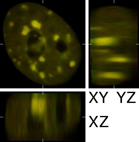
small mainly because of photo-toxicity (the living        lows us to get reasonable computational times even
specimen is harmed by the light) and photo-bleaching      for 3D image sequences.
(the intensity of fluorescent markers fades while be-         The rest of the paper is organized as follows: The
ing exposed to the light). However, it is usually pos-    variational optical flow methods are described in Sec-
sible to find a reasonable compromise between those       tion 2. Section 3 is devoted to the experiments and re-
restrictions and adjust the image acquisition so that     sults obtained for synthetic and real biomedical data.
the displacement of objects between two consecutive
snapshots is not more than ten pixels.
    There are two types of tasks to be solved in this     2 OPTICAL FLOW
field. First, the global movement of objects should
be corrected before subsequent analysis of an intra-      In this section, we describe the basic ideas of varia-
cellular movement. This goal is often achieved us-        tional optical flow methods and in particular the meth-
ing common rigid registration methods (Zitová and        ods which will be tested in Section 3.
Flusser, 2003). A fast 3D point based registration            Let two consecutive frames of image sequence be
method (Matula et al., 2006) was recently proposed        given. Optical flow methods compute the displace-
for the global alignment of cells.                        ment vector field which maps all voxels from first
    The second task is to estimate local changes in-      frame to their new position in the second frame. Al-
side the objects. This task is more complex. The ob-      though several kinds of strategies exist for optical
jects inside the cells or nuclei can move in different    flow computation (Barron et al., 1994), we take only
directions. One object can split into two or more ob-     the so-called variational optical flow (VOF) methods
jects and vice versa. Moreover, an object can appear      into our considerations. They currently give the best
or disappear during the experiment. Therefore, this       results (in terms of error measures) (Papenberg et al.,
task requires computation of dense motion field be-       2006; Bruhn and Weickert, 2005) and come out from
tween two consecutive snapshots. Manders et. al. has      transparent mathematical modeling (the flow field is
used block-matching (BM3D) algorithm (de Leeuw            described by energy functional). Furthermore, they
and van Liere, 2002) for this purpose in their study      produce dense flow fields and are invariant under ro-
of chromatin dynamics during the assembly of inter-       tations.
phase nuclei (Manders et al., 2003). Their BM3D               The first prototype of VOF method was proposed
algorithm is rather slow. It is similar to basic optic    in (Horn and Schunck, 1981). Horn and Schunck
flow methods but it does not comprise any smooth-         used the grey value constancy assumption which as-
ness term.                                                sumes that the grey value intensity of the moving ob-
    We study latest optical flow methods (Bruhn,          jects remains the same and homogenous regulariza-
2006) for estimation of intracellular movement in this    tion which assumes that the flow is smooth. We will
paper. Up to our best knowledge, nobody investi-          describe their method first, because even the most so-
gated the application of these state-of-the-art meth-     phisticated methods available are based on the funda-
ods in live-cell imaging. The simple ancestors of         mental ideas of Horn and Schunck method.
these methods, which can reliably estimate one pixel          Let Ω4 ⊂ R4 denote the 4-dimensional spatial-
motion, were successfully used for lung motion cor-       temporal image domain and f (x1 , . . . , x4 ) : Ω4 → R
rection (Dawood et al., 2005). The examined meth-         a gray-scale image sequence, where (x1 , x2 , x3 ) is a
ods are able to reliably estimate the flow larger than    voxel location within a image domain Ω3 ⊂ R3 and
one pixel. They can produce piece-wise smooth flow        x4 ∈ [0, T ] denotes the time. Moreover, let’s assume
fields which preserve the discontinuities in the flow     that ∆x4 = 1 and u = (u1 , u2 , u3 , 1) denotes the un-
on object boundaries. These properties are needed for     known flow. The grey value constancy assumption
estimation of local divergent motion which occur in       says
live-cell imaging. We have extended state-of-the-art       f (x1 +u1 , . . . , x3 +u3 , x4 +1)− f (x1 , . . . , x4 ) = 0 (1)
optical flow methods into three dimensions. Espe-
cially, we focused on 3D extension of recently pub-       Optic flow constraint (OFC) is obtained by approxi-
lished optical flow methods for large displacements       mation of (1) with first-order Taylor expansion
(Papenberg et al., 2006). We tested these methods on                   fx1 u1 + fx2 u2 + fx3 u3 + fx4 = 0,              (2)
synthetic as well as real data and compared their be-
haviour and performance. Our experiments identify         where fxi is partial derivative of f . Equation (2) with
the optical flow methods which can be used in live cell   three unknowns has obviously more than one solu-
imaging. We used the efficient numeric techniques for     tion. Horn and Schunck assumed only smooth flows
the optical flow computations (Bruhn, 2006). This al-     and they therefore penalized the solutions which have
large spatial gradient ∇3 ui where i ∈ 1, 2, 3 and ∇3 de-        where
notes the spatial gradient. Thus, the sum ∑3i=1 |∇3 ui |
for every voxel should be as small as possible. We                       ΨD (s) =    s2 + ε2D      ΨS (s) =    s2 + ε2S
get following variational formulation of the problem
if we combine these two considerations together:                 and εD , εS are reasonably small numbers (e.g. εD =
                Z                                                0.01). Note that the data term consists of non-
   EHS (u) =         ( fx1 u1 + fx2 u2 + fx3 u3 + fx4 )2         linearized grey value constancy assumption (1). This
                 Ω                                               allows to correct estimate of the large displacements.
                            3                              (3)
                                                                 Moreover, the CLG method uses the non-quadratic
                     + α ∑ |∇3 ui |2 dx
                                                                 penalizers ΨD (s) and ΨS (s) and therefore it is ro-
                          i=1
                                                                 bust with respect to noise and outliers. Nevertheless,
The optimal displacement vector field minimizes en-              these concepts make the minimization of (5) quite
ergy functional (3). The OFC and the regularizer are             complex. We use the multi-scale warping based ap-
squared, the α parameter has the influence on the                proach, which proposed in (Papenberg et al., 2006),
smoothness of the solution. The two terms which                  for minimization of (5). The multigrid numerical
form the functional are called data and smoothness               framework for this task was extensively analyzed in
term. Following the calculus of variations (Gelfand              (Bruhn, 2006; Bruhn and Weickert, 2005).
and Fomin, 2000), the minimizer of (3) is a solution                 The second tested method consists of robust data
of Euler-Lagrange equations                                      term and anisotropic image driven smoothness term
                                                                 (Nagel and Enkelmann, 1986). We denote this
      0 = fx21 u1 + fx1 fx2 u2 + fx1 fx3 u3 + fx1 fx4            method RDIA. Its energy functional is defined:
          + α div(∇3 u1 )                                                        Z
      0 = fx1 fx2 u1 + fx22 u2 + fx2 fx3 u3 + fx2 fx4              ERDIA (u) =          ΨD (| f (x + u) − f (x)|2 )
                                                           (4)                      Ω
          + α div(∇3 u2 )                                                                     3
      0 = fx1 fx3 u1 + fx2 fx3 u2 + fx23 u3 + fx3 fx4                                   + α ∑ (∇3 u
                                                                                                   i PNE (∇3 f )∇3 ui ) dx
          + α div(∇3 u3 )                                                                    i=1
                                                                                                                          (6)
with reflecting Neumann boundary conditions. div(x)
is the divergence operator. The system (4) is usu-               where PNE (∇3 f ) is projection matrix perpendicular to
ally solved with common numerical methods like                   ∇3 f defined as
Gauss-Seidel or SOR. The bidirectional full multigrid                                            ⎛            ⎞
(Briggs et al., 2000) framework for computations of                                     1          a b c
                                                                         PNE =                   ⎝ b d e ⎠          (7)
VOF methods was proposed in (Bruhn et al., 2005).                                2|∇3 f |2 + 3ε2
The computations with multigrid methods are by or-                                                 c e f
ders of magnitude faster than the classic Gauss-Seidel
                                                                 where
or SOR methods.
    Now we describe the VOF methods which will be                        a = fx22 + fx23 + ε2      d = fx21 + fx23 + ε2
tested in Section 3. The current state-of-the-art VOF                    b = − f x1 f x2           e = − f x2 f x3
methods are still similar to their Horn-Schunck pre-                     c = − f x1 f x3           f = fx21 + fx22 + ε2
cursor. Their energy functional consists of data and
smoothness term. The combined local-global (CLG)                 The ε is reasonably small number (e.g. ε = 0.01).
method for large displacements proposed in (Papen-               The only difference between CLG and RDIA method
berg et al., 2006) is the first method which we have             is the smoothing term. RDIA method smoothes the
tested. This method produces one among the most                  flow with respect to underlying image. The image
accurate results (Bruhn, 2006). We assume that it will           data in live-cell imaging are often low contrast due
be suitable for our data, because it produces smooth             to the limitations of the optical setup. We assume that
flow fields and simultaneously flow fields with dis-             this smoothing term can help with processing of such
continuities. The energy functional of CLG method                data. The same minimization approach can be used as
is defined as:                                                   for the CLG method.
                      Z                                              The third and fourth tested method are variants of
       ECLG (u) =           ΨD (| f (x + u) − f (x)|2 )          the previous two. We add the gradient constancy as-
                        Ω
                                                         (5)   sumption to the data term. This should provide us bet-
                                        3
                            + αΨS      ∑ |∇3 ui |2 dx            ter results on image sequences which fade out with in-
                                                                 creasing time. The energy functional of CLG method
                                      i=1
with gradient constancy assumption is defined as
ECLGG (u) =
Z
ΨD (| f (x + u) − f (x)|2 + γ(|∇ f (x + u) − ∇ f (x)|2 ))
Ω
3
+ αΨS ∑ |∇3 ui |2 dx
i=1
(8)
The variant of RDIA method with gradient constancy
assumption is defined as
ERDIAG (u) =
Z
ΨD (| f (x + u) − f (x)|2 + γ(|∇ f (x + u) − ∇ f (x)|2 )) Figure 1: Generation of artificial data. We use two-layered
Ω
approach. Both artificial frames are generated from the real
3
input frame. The second frame is almost identical to the real
+ α ∑ (∇3 u
i PNE (∇3 f )∇3 ui ) dx one. The first frame is the backward registered copy of sec-
i=1
ond frame. The artificial ground-truth flow field is used for
(9) the backward registration. The background and foreground
where γ is the parameter which controls the influence movements are independent. (top left) Real input frame.
of gradient constancy assumption. Note that the gra- (top right) Cell nucleus mask (background) in white, object
mask (foreground) in red. (bottom left) Second artificial
dient constancy assumption is again included in the
frame. (bottom right) First artificial frame (red channel)
non-linearized form. superimposed over second frame (green channel).
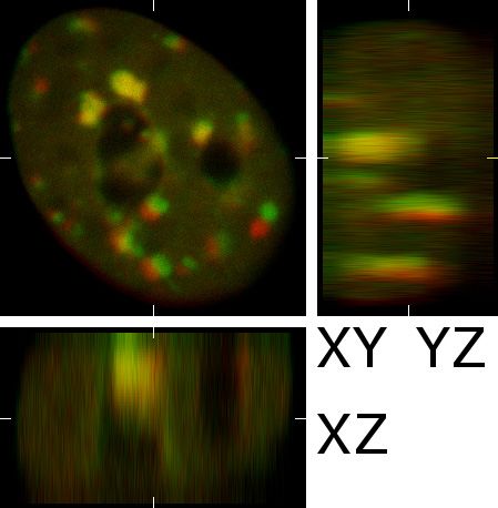
1994) according to the generated flow field. This flow
3 RESULTS AND DISCUSSION determines the movement and becomes the ground-
truth flow. The flow field determines the movement
In this section, we test the behaviour of CLG, uniquely. Thus, it becomes the ground-truth flow field
RDIA, CLGG and RDIAG methods on artificial and between these two frames and can be used for testing
real image data. We measure their performance on purposes. Owing to the property of the backward reg-
live-cell image sequences with large local displace- istration technique, the first frame represents the in-
ments. Moreover, we present the results of the meth- put real image before the movement while the second
ods on image sequences with combined global rigid frame represents it after the movement. Therefore, the
(translation, rotation) and local displacements. We second frame is similar to the real input image. The
present the results on both two and three dimensional generation process is illustrated in Fig. 1.
data. Finally, we discuss the computational time and The first experiment was performed on artificial
storage demands. two dimensional data. We prepared a data set of arti-
The ground-truth flow fields are needed for the ficial images with large local displacements. The data
evaluation purposes. Obviously, they are not avail- set consisted of six different frame couples. The size
able for real image sequences. Therefore, we gener- of input frames was 400 × 400 pixels. The number of
ate the artificial data with artificial flow fields from objects which moved inside the nucleus varies from
the real image data. We use the two-layered approach seven to eleven. The size of the individual translations
in which user-selected foreground is locally moved vectors varies from 1.2 to 11.3 pixels. According to
and inserted into an artificially generated background. the literature, the input frames were filtered with gaus-
Hence, our generator requires one real input frame, sian blur filter with standard deviation σ = 1.5. We
the mask of the cell (the background) and the mask performed a parametric study over α parameter for
of the objects (the foreground). Both first and sec- four tested methods over whole data set. The results
ond frames are generated in two steps. First, the were compared with respect to average angular error
foreground objects are extracted, an artificial back- (AAE) (Fleet and Jepson, 1990) where angular error
ground is generated and the rigid motion is applied is defined as
on background and foreground separately. Second, ⎛ ⎞
every foreground object is translated independently (u ) (u ) + (u ) (u ) + 1
arccos ⎝ ⎠
1 gt 1 e 2 gt 2 e
on each other and finally inserted into the generated
background. The movements were performed by us- ((u1 )gt + (u2 )gt + 1)((u1 )2e + (u2 )2e + 1)
2 2
ing backward registration technique (Lin and Barron, (10)where (ui )gt , (ui )e denote the i-component of ground- 26
AAE of CLGg method
AAE of CLG method
24
truth and estimated vector, respectively. There were 22
two coupled goals behind this experiment. We wanted 20
AAE
to identify the best method by the mean of AAE and 18
at the same time find suitable setting of α parameter.
16
14
The results are presented in Fig. 2. The AAE was 12
2 4 6 8 10 12 14
computed for each run of particular method with par- α parameter
ticular α. Then, the averages of AAE over the frame 18
AAE of RDIAg method
pairs in the data set were computed. These averages 17 AAE of RDIA method
16
are depicted in the graphs in Fig. 2. The AAE was 15
AAE
computed only inside the moving objects. We can see 14
that all methods perform reasonably well. The CLG 13
method is outperformed by the RDIA method. The 12
11
gradient variant of CLG provided better results than 50 100 150
α parameter
200 250 300
the simple CLG method. The RDIAG method is not
14
depicted in the graph because we noticed that its re- 13
AAE of CLGg method
AAE of CLG method
sults depended on data and the average value was bi- 12
ased. It was slightly better than simple RDIA method
AAE
11
in some cases. But, it was slightly worse in other 10
cases. 9
8
4 6 8 10 12 14
16
AAE of CLGg method α parameter
14 AAE of CLG method
12 12.5
AAE of RDIAg method
10 12 AAE of RDIA method
AAE
11.5
8
11
6
AAE
10.5
4
10
2 9.5
5 10 15 20
α parameter 9
8.5
50 100 150 200 250 300
2.38
AAE of RDIA method α parameter
2.36
2.34
2.32
2.3 Figure 3: The dependency of average angular error on α
2.28
AAE
2.26 parameter. The methods were tested on artificial image
2.24
2.22 data with global movement (translation up to 5 pixels, ro-
2.2
2.18
tation up to 4 degrees) and large local displacements up to
2.16
50 100 150 200 250 300
11.3 pixels. (top) CLG and CLGG method. (upper cen-
α parameter ter) RDIA and RDIAG method. Majority of local displace-
ments have the same direction as compared to global move-
Figure 2: The dependency of average angular error on α ment (top, upper center). (lower center) CLG and CLGG
parameter. The methods were tested on artificial image data method. (bottom) RDIA and RDIAG method. Majority
with large local displacements up to 11.3 pixels. (top) CLG of local displacements has different direction than global
and CLGG method. (bottom) RDIA method. movement (lower center, bottom).
The goal of the second experiment was to examine
the performance of the tested methods on sequences global translation the results fell into the first group
with combination of global and local movement. We and vice versa. The AAE was computed on the cell
again prepared a dataset with artificial frame pairs. nucleus mask (see the Fig. 1) in this experiment. The
Image size and other input sequence properties were results for both groups are illustrated in Fig. 3.
the same as in the previous experiment. The cell nu- We tested the methods with best parameter set-
clei were transformed with global translation (up to tings on real three dimensional data in the third ex-
5 pixels) and rotation (up to 4 degrees). After that periment. We computed the displacement field of two
the local displacement were applied on the foreground input frames of human HL-60 cell nucleus with mov-
object inside. It becomes clear from our experiments ing HP1 protein domains. There are global as well as
that we should divide the data into two groups. The local movements in the frame pair (see Fig. 4). We es-
results of the computations were influenced by the timated the flow with RDIA method, α was set to 100.
following fact. If the majority of objects inside the The size of the input frames was 276×286×106. The
cell nucleus moved in the direction similar to the results are illustrated in Fig. 4.The VOF methods were implemented in C++ lan-
guage and tested on common workstation (Intel Pen-
tium 4 2.6 GHz, 2 GB RAM, Linux 2.6.x). We use the
multigrid framework (Bruhn, 2006) for numerical so-
lution of tested VOF methods. The computations on
two 3D frames of size 276 × 286 × 106 took from 700
to 920 seconds and needed 1.5 GB of RAM. Compu-
tations on two 2D frames of size 400 × 400 took from
13 to 16 seconds and needed 13 MB of RAM.
3.1 Discussion
We found out that the RDIA methods produce slightly
better results than the CLG methods (with respect to
AAE) in both experiments on synthetic live-cell im-
age data. Moreover, RDIA methods are less sensi-
tive to α parameter setting. It became clear that the
smoothing term of RDIA method is more suitable for
the low contrast image sequences. The computed flow
field can be easily oversmoothed by the CLG meth-
ods, because they consider the moving objects to be
outliers in the data by particular parameter settings
(larger α).
The use of “gradient” variants of tested method
can slightly improve their performance on live-cell
image data. On the other hand, there is no warranty
that the result will be always better. Actually, the
RDIA method seems to be more sensitive to α param-
eter when using its “gradient” variant. Surprisingly,
the expected improvement of “gradient” variants was
not significant even for fading out sequences. We sup-
pose that the gradient constancy assumption does not
help a lot, because the decrease of the intensities be-
tween two consecutive frames is not big. To sum it up,
the 2D tests show that the RDIA method is the most
suitable for our data. Therefore, we used it for the ex-
periment on the 3D real image data. The backward
registered results show perfect match on xy-planes.
The match in xz and yz planes is a little bit worse.
This is caused by the lower resolution of the micro-
scope device in the z axis.
The bleeding-edge multigrid technique allowed us
to get the flow fields in reasonable times even for 3D
(up to 15 minutes for one frame pair). Small data sets
which consist of only tens of frames of several cells
can be analyzed in order of days on one common PC.
Larger data sets as well as parametric studies in 3D
Figure 4: Experiment with real 3D data. Frame
size 276 × 286 × 106. xy, xz and yz cuts on position
should be analyzed on a computer cluster.
(138, 143, 53) are shown. (top) First input frame. (cen-
ter) First input frame (red channel) superimposed on sec-
ond frame (green channel). Correlation is 0.901. (bottom)
The RDIA method with α = 100 computes the flow field.
4 CONCLUSION
Backward registered second frame (green channel) is su-
perimposed onto first frame (red channel). Correlation is We studied state-of-the-art variational optical flow
0.991. methods for large displacement for motion trackingof fluorescently labeled targets in living cells. We fo- Chalfie, M., Tu, Y., Euskirchen, G., Ward, W. W., and
cused on 2D as well as 3D images. Up to our best Prasher, D. C. (1994). Green fluorescent protein as a
knowledge, we tested those methods first time in the marker for gene-expression. Science, 263(5148):802–
805.
literature for three dimensional image sequences.
We showed that these methods can reliably es- Dawood, M., Lang, N., Jiang, X., and Schäfers, K. P.
(2005). Lung motion correction on respiratory gated
timate large local divergent displacements up to ten 3d pet/ct images. IEEE Transactions on Medical
pixels. Moreover, the methods can estimate the global Imaging.
as well as local movement simultaneously. The vari-
de Leeuw, W. and van Liere, R. (2002). Bm3d: Motion es-
ants of CLG and RDIA method with gradient con- timation in time dependent volume data. In Proceed-
stancy assumptions did not bring significant improve- ings IEEE Visualization 2002, pages 427–434. IEEE
ment for our data. The RDIA method produced the Computer Society Press.
best results in our experiments. We achieved reason- Fleet, D. J. and Jepson, A. D. (1990). Computation of com-
able computation times (even for three dimensional ponent image velocity from local phase information.
image sequences) using the full bidirectional multi- Int. J. Comput. Vision, 5(1):77–104.
grid numerical technique. Gelfand, I. M. and Fomin, S. V. (2000). Calculus of Varia-
We plan to perform larger parametric studies on tions. Dover Publications.
three dimensional data. This studies need to be per- Horn, B. K. P. and Schunck, B. G. (1981). Determining
formed on computer cluster or grid because of com- optical flow. Artificial Intelligence, 17:185–203.
putational demands. Owing to the achieved results, Kozubek, M., Matula, P., Matula, P., and Kozubek, S.
we also feel confident in building a motion tracker as (2004). Automated acquisition and processing of
an application based on tested methods. By analyz- multidimensional image data in confocal in vivo
ing computed flow field one can extract important bi- microscopy. Microscopy Research and Technique,
64:164–175.
ological data regarding the movement of intracellular
structures. Lin, T. and Barron, J. (1994). Image reconstruction error
for optical flow. In Vision Interface, pages 73–80.
Manders, E. M. M., Visser, A., Koppen, A., de Leeuw,
W., van Driel, R., Brakenhoff, G., and van Driel, R.
ACKNOWLEDGEMENTS (2003). Four-dimensional imaging of chromatin dy-
namics the assembly of the interphase nucleus. Chro-
This work was partly supported by the Ministry of mosome Research, 11(5):537–547.
Education of the Czech Republic (Grants No. MSM- Matula, P., Matula, P., Kozubek, M., and Dvořák, V. (2006).
0021622419 and LC-535) and by Grant Agency of the Fast point-based 3-d alignment of live cells. IEEE
Czech Republic (Grant No. GD102/05/H050). Transactions on Image Processing, 15:2388–2396.
Nagel, H. H. and Enkelmann, W. (1986). An investigation
of smoothness constraints for the estimation of dis-
placement vector fields from image sequences. IEEE
REFERENCES Trans. Pattern Anal. Mach. Intell., 8(5):565–593.
Papenberg, N., Bruhn, A., Brox, T., Didas, S., and Weick-
Barron, J. L., Fleet, D. J., and Beauchemin, S. S. (1994). ert, J. (2006). Highly accurate optic flow computa-
Performance of optical flow techniques. Int. J. Com- tion with theoretically justified warping. International
put. Vision, 12(1):43–77. Journal of Computer Vision, 67(2):141–158.
Briggs, W. L., Henson, V. E., and McCormick, S. F. (2000). Zitová, B. and Flusser, J. (2003). Image registration meth-
A multigrid tutorial: second edition. Society for In- ods: a survey. 21(11):977–1000.
dustrial and Applied Mathematics, Philadelphia, PA,
USA.
Bruhn, A. (2006). Variational Optic Flow Computation:
Accurate Modelling and Efficient Numerics. PhD the-
sis, Department of Mathematics and Computer Sci-
ence, Universität des Saarlandes, Saarbrücken.
Bruhn, A. and Weickert, J. (2005). Towards ultimate motion
estimation: Combining highest accuracy with real-
time performance. In Proc. 10th International Confer-
ence on Computer Vision, pages 749–755. IEEE Com-
puter Society Press.
Bruhn, A., Weickert, J., and Schnörr, C. (2005). Variational
optical flow computation in real time. IEEE Transac-
tions of Image Processing, 14(5).You can also read