Drone Detection and RCS Measurements with Ubiquitous Radar
←
→
Page content transcription
If your browser does not render page correctly, please read the page content below
Drone Detection and RCS Measurements
                        with Ubiquitous Radar

         Álvaro Duque de Quevedo, Fernando Ibañez Urzaiz, Javier Gismero Menoyo, Alberto Asensio López
                    Information Processing and Telecommunications Center. Universidad Politécnica de Madrid
                                                       Madrid, Spain
                     aduque@gmr.ssr.upm.es, f.ibanez@upm.es, javier@gmr.ssr.upm.es, vera@gmr.ssr.upm.es

    Abstract— This paper presents experimental results on             from weather or lighting conditions, and their suitability for the
commercial-drone detection with a ubiquitous frequency                operational needs in drone detection [2]). In spite of this, the
modulated continuous wave (FMCW) radar system, working at             detection of a commercial micro-UAV is a real challenge for
8.75 GHz (X-band). The system and its main blocks are briefly         radar technology due mainly to its small size and plastic-made
introduced. Subsequently, the document presents the chosen            and low-reflective materials translating to its very low Radar
scenario for the tests, and shows the results of the offline signal   Cross Section (RCS) and its ability to fly slowly at ground
processing, achieving a DJI-Phantom-4 detection at a range up to      level, making its echoes to compete with high clutter signals.
2 km. The results are illustrated with range-Doppler matrices
and detection figures. Range, speed and azimuth accuracies are            This paper introduces our RAD-DAR: a small, quick-to-
discussed, considering the drone GPS data. Finally, the paper         deploy and low-powered radar demonstrator system, based on
introduces a statistical radar-cross-section (RCS) study based on     the ubiquitous radar concept [3], which is able to detect and
the processed data, in order to classify the drone as a Swerling      track a small commercial drone flying at a range of 2 km. Our
target, and discusses the drone average RCS.                          first experimental results, introduced in [4], showed the
                                                                      feasibility of achieving strong range-speed association with the
    Keywords— drone detection; persistent radar; radar cross-         developed demonstrator. This article presents the results of new
sections; radar detection; radar remote sensing; RPA detection;       tests (Sec. V) focused on drones instead of cars, with very
UAV detection; ubiquitous radar.
                                                                      promising outcomes. Collected data have been also employed
                                                                      in order to study the drone RCS, as will be seen in Sec. VI.
                       I.    INTRODUCTION
    We are currently living a boom in drone use, for not only             II.   X-BAND UBIQUITOUS RADAR: SYSTEM DESCRIPTION
defense purposes but also commercial, professional, and
entertainment. This rise is based on the great commercial offer,      A. Ubiquitous radar concept
which is constantly growing, the relatively affordable cost of            The system presented in this article is a ubiquitous radar
drones, its effectiveness in surveillance tasks and in package        demonstrator [3], which always stares at the whole surveillance
delivering, and the inherent allure of the easy handling of this      scene with a wide transmitted beam. An 8-channel digital array
cutting-edge technology. Drones provide a new form of                 receives the echoes, digitizes, and stores them for further
entertainment for everyone with amazing multimedia results.           processing. The system uses multiple simultaneous beams
Maybe, one day, seeing drones will be as normal as seeing mail        generated on reception by means of digital beamforming, in
trucks on the road [1], or any toy at home.                           order to achieve the required azimuthal coverage.
    However, this quick evolution also implies the rise of a new          The absence of scanning (mechanical or electronic) allows
threat to global security from a number of points of view. On         for reaching an optimal trade-off between the dwell time and
the one hand, the right to privacy of individuals may be easily       the refreshing rate of target data. This enables the system to
compromised, and their security could be put at risk because of       adapt in order to detect and track low radar cross section targets
the proximity of these aircrafts in flight. Furthermore, drones       with slow dynamics (e.g. drones), without degrading abilities
represent a potential risk of plane crash when passing through        to detect other faster and bigger targets (e.g. vehicles, planes).
protected airspace or flying near airports. Finally, the same
mentioned usability and the easy access to these systems may
result in an advantage for terrorists, who can commit their                                                    Synthesized Rx beams
attacks in a more effective and less exposed way.                                    Tx beam

   Hence, on a par with this drone boom, the competent
authorities have rushed to upgrade the attendant legislation and
many systems for drone detection and shoot-down have arisen.
Amongst all of them (e.g. audio- or video-based systems),                                        RAD-DAR
radar systems are positioning themselves one step ahead
because of their inherent advantages (e.g. its independence           Fig. 1 Ubiquitous Radar working principle.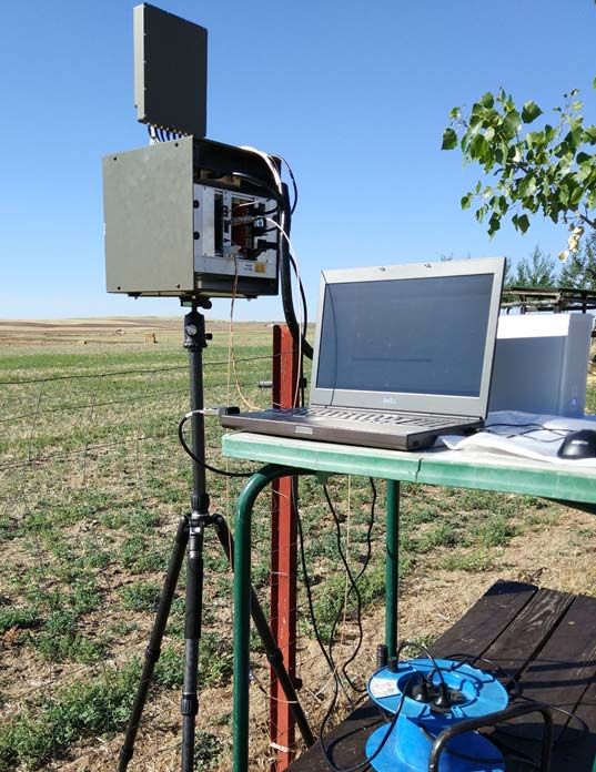
Tx Antenna       Rx Antenna, 8 Receivers                                                                                                           L
                                                                                                                                            fast-time, samples
                                                                                                                                                  (range)
                                                                                                                OFF-LINE RADAR DATA
                                                                                                                                                          1
                                                                                                                     PROCESSOR                           1

                                                                                                                 Traking                     channels
                                                                                                                                            (azimuth)
                                                                                                                 algorithms                              M
                                                                                                                                                              1            N
                                                                                                                                                slow-time, ramps (Doppler, speed)

                                             RAD – DAR                                        8-channel                               CA – CFAR                      Beamforming M
                                                                                               Digitizer                                       T                  win     &
                                                                                                                       Plot                                           Mononopulse
                                LO                                                                                                        Detection
                                                                                                                    extraction
                                                                                        Control &
                    Transmitter                                                         Acquisition
                                            8 ch Digitizer             PC
                                                                                        Software                     win      1st FFT L            win   2nd FFT N
                                            PCIe Express       (Signal Processor,
           Power supply   8.75GHz                               Data Processor)
                                  Clock                                                ACQUISITION SUBSYSTEM                  OFFLINE RADAR SIGNAL PROCESSOR
                      Signal
                    Generator     Trigger
                                                                                     Fig. 3 Block diagram of the RAD-DAR Software, and data cube.

Fig. 2 Block diagram of the RAD-DAR Hardware.                                       pointing angles θ between -40º and +40º (see Fig. 4). To do
                                                                                    this, a phase increment is applied to each received signal,
B. Hardware description                                                             according to the inter-element spacing and the pointing angle
    Fig. 2 shows a diagram of the radar demonstrator. The                           desired [7], [4], [5]. By adding the 8 phase-shifted signals,
RAD-DAR employs a programmable signal generator to obtain                           range-Doppler matrices are generated for each pointing angle.
a frequency modulated continuous wave (FMCW), on a
                                                                                        In order to improve the azimuth accuracy, the Signal
frequency band centered at 8.75 GHz (X-band) with a
                                                                                    Processor performs a monopulse technique. After generating
maximum bandwidth of 500 MHz, and clock and trigger
                                                                                    the sum signal at the beamforming process, a difference signal
signals. A transmitter amplifies the signal up to 5W and
                                                                                    is also obtained for each pointing angle, θ, by subtracting
generates the Local Oscillator (LO) sample for subsequent
                                                                                    channel 5-8 signals from channel 1-4 signals. The quotient
demodulation. The 8 receiving antennas and the transmitting
                                                                                    between the magnitudes of difference signal (∆) and sum signal
one are designed with microstrip technology [5].
                                                                                    (Σ) yields the Monopulse Function [8, Sec. 9.2]. The azimuth
                                                                                    accuracy improvement is achieved by comparing the
C. Software description                                                             Monopulse Function values obtained from signal processing,
    The signal from 8 receivers is acquired by a commercial 8-                      using data cubes, with the corresponding Monopulse Function
channel digitizer [6] connected to a computer by a PCIe port. A                     values obtained from anechoic-chamber data [8], [4].
Matlab script has been developed to carry out the digitizer
control. This Signal Acquisition Subsystem captures data                                3) Decision and plot extraction
arranging them into cubes (Fig. 3) for a posterior 3D                                   A Cell-Averaging Constant False Alarm Rate (CA-CFAR)
processing. These three dimensions are range (the system                            technique [7] is applied at detection stage in order to obtain a
captures L samples per trigger), time (N ramps are acquired)                        binary cube with detections. This is carried out by comparing
and azimuth (M channels, M = 8).                                                    the signal power at a range bin with an adaptive threshold
                                                                                    calculated as the average signal power of its adjacent cells
   The block diagram in Fig. 3 is a quick description of the                        (reference cells). Each target detection is turned to a plot (a
Radar Software, including the Acquisition Subsystem, the                            single-point detection) by computing its center of mass, usually
Radar Signal Processor, and the Data Processor.                                     referred to as centroid [9]. Thus, after detection, a list of plots
    The offline Radar Signal Processor, implemented with                            is obtained, each one containing information about range,
Matlab, works with the data cubes from the Acquisition                              speed, azimuth, received signal power and time.
Subsystem. It performs a 3D processing (Two-dimension Fast                             A Data Processor, which is currently under development,
Fourier Transform, beamforming and monopulse) and a                                 obtains tracks from plots which belong to a tracked target.
detection and plot extraction stage.
    1) Two-dimension Fast Fourier Transform (2D FFT)
    By means of a FMCW waveform [4], target range
information lies in the “beating frequency” (fb), which is the
difference between transmitted and reflected frequencies. A
Fast Fourier Transform (FFT) is applied to the L dimension
(see Fig. 3) in order to obtain the beating frequency, and so the
range information. A second FFT, performed over the N
dimension, provides Doppler information (speed) if care is
taken to ensure the synchronism during the acquisition process.
    2) Beamforming and Monopulse
    On the basis of the signals coming from the 8 channels, the
system synthesizes 5 reception beams corresponding to                               Fig. 4 RAD-DAR synthesized beams by Beamforming.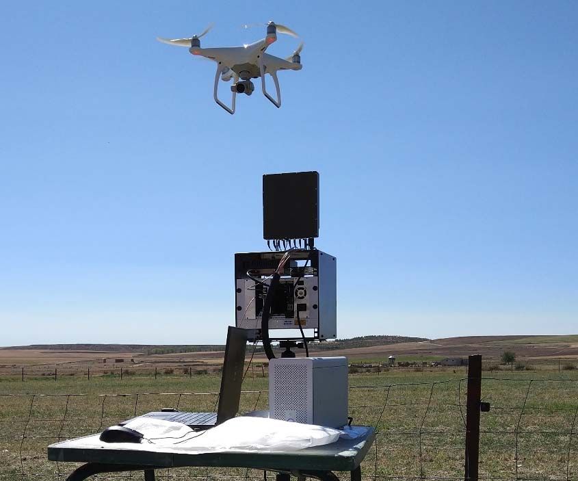
III. DRONE DETECTION TEST SETUP
TABLE I. DJI PHANTOM 4 MAIN SPECIFICATIONS
A. Target Characteristics Weight (propellers and battery included) 1380 g
The tests described in this paper were performed with a Diagonal length (propellers not included) 350 mm
commercial micro-drone (also referred to as micro- Unmanned Maximum speed 20 m/s (72 km/h)
Aerial Vehicle, micro-UAV, or micro- Remotely Piloted Maximum flying height (above sea level) 6000 m
Positioning system GPS/Glonass
Aircraft, micro-RPA), DJI Phantom 4 [10], designed for both
Maximum flying time (battery life) 28 minutes
private and professional use. Table I shows its main features. Maximum range (remote control range) 5 km
The main material of the drone body is plastic, the
propellers are made with glass fiber reinforced composite and TABLE II. FIELD TESTS: DRONE OUTWARD FLIGHT
and the four rotors are made of carbon fiber and plastic as well. Flight Control Mode Manual
A considerable amount of literature has been published on Flight time 271 s
drones cross section. Refs [11], [12] and [13] show results on Average speed 8.26 m/s (29.72 km/h)
RCS obtained by means of anechoic chamber measurements or Standard deviation of the speed 0.57 m/s (2.04 km/h)
simulation, of a DJI Phantom 2, which is similar to Phantom 4 Average altitude (over the floor) 21.6 m
Standard deviation of the altitude 0.1 m
in terms of weight, size, materials and shape. There is a view
widely held in these articles that a Phantom drone may be
TABLE III. FIELD TESTS: DRONE RETURN FLIGHT
modeled as a Swerling 1 target (SW1) with an average RCS of
approximately 0.01m2 (-20 dBsm). Flight Control Mode Auto (Go to Home)
Flight time 237 s
This drone is able to record its telemetry data during a Average speed 9.96 m/s (35.85 km/h)
flight. These data (e.g. GPS coordinates, range, speed) are Standard deviation of the speed 0.06 m/s (0.22 km/h)
collected at 10 Hz sample frequency and easy to export for Average altitude (above ground level) 30.2 m
further processing. Standard deviation of the altitude 0.2 m
B. Field-test scenario C. Radar setup
The selected scenario for the field tests is a farm located at The performed drone-detection experiments were carried
a village in the province of Ávila, Spain. Its geographical out with a radar setup summarized by Table IV, Table V, and
coordinates are 40°49'47.3"N 4°48'00.4"W [14]. The system Table VI, introducing waveform, operative and acquisition
was installed over an emplacement with entirely unobstructed parameters.
line of sight extended up to 5 km.
As can be seen in these tables, it can be expected that the
As Fig. 5 shows, the drone described a round trip for these system achieves a strong range-speed association due to the
tests. The outward flight was driven by a pilot, by means of the corresponding resolutions. The dwell time of 0.17s allows the
manual mode of the drone remote control. The return flight radar to reach a high speed resolution and an enough
was carried out in automatic “Go to home” mode. The integration time to raise the Signal-to-Noise Ratio (SNR), thus
maximum range achieved by the drone was 2 km. Table II and achieving the desired detection range. The maximum
Table III summarize the data of these flights. unambiguous range and the Doppler ambiguity seem to be
In view of these flight data, it is easy to conclude that the
return flight is the best to assess the radar performance, since
drone managed to keep a quasi-constant trajectory with low
speed deviation by means of that automatic control mode.
Thus, Section IV will focus in that radar results of the return
flight, although the outward flight will be also introduced.
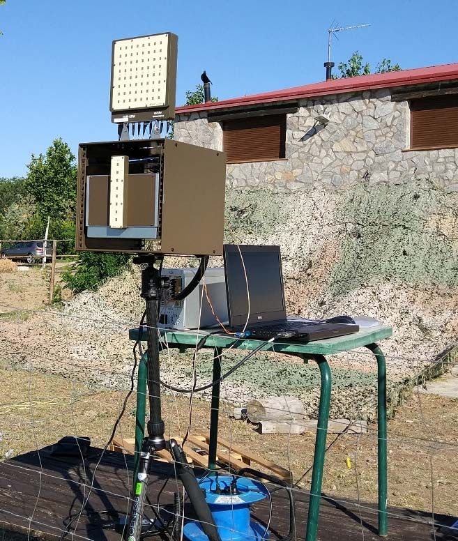
Fig. 6 shows the radar system installed for the test. There
were some birds of prey at the coverage area, which sometimes
appeared in the captured data. Although the studied data for
this paper are focused on the drone flight, future articles will
deal with bird detection, tracking, and micro-doppler studies.
Fig. 5 Field-test scenario. Fig. 6 RAD-DAR and drone, at site for field testTABLE IV. WAVEFORM PARAMETERS V. DRONE DETECTION RESULTS
Radar frequency (f1) 8.75 GHz The drone was detected and tracked from the beginning to
Bandwidth (Δf) 200 MHz the end of the flights, achieving a detection-range up to 2 km,
Ramp period (Tm) 350 μs
with Pd > 0.7, as was predicted in Section IV.
Ramp frequency (fm) 2.86 kHz
TABLE V. UBIQUITOUS RADAR PERFORMANCE A. Linear target path (return flight)
Range Resolution (ΔR) 0.878 m
Fig. 8 shows a range-Doppler matrix with raw data (after
Maximum unambiguous range (Rmna) 3598 m (fb = 16 MHz) 2D FFT and beamforming) with pointing angle θ = 0º, where
Doppler Resolution 5.58 Hz, 0.096 m/s, 0.34 km/h clutter can be appreciated at zero Doppler along every range
Doppler ambiguity 1.4 KHz, 24.5 m/s, 88.1 km/h bins. When zooming (Fig. 9) the drone can be found at
0.83km-range and 36km/h-speed bins. This figure corresponds
TABLE VI. ACQUISITION PARAMETERS to the cube number 200/400 of the return flight test (negative
Number of samples per ramp (L) 8192
drone speed because it is approaching to the radar system).
Number of integrated ramps (N) 512 Fig. 10 shows the detected drone speed vs distance.
Number of channels (M) 8 Average detected speed was 35.95 km/h with a standard
Number of range bins (nBins) 4096 (3598 m)
Dwell time 0.1792 s
deviation (STD) of 0.19 km/h, which is similar to the GPS data
Number of synthesized beams 5 (Table III). The average-speed error, comparing radar
Sample rate (fs) 32 MHz measurements with GPS data, is 0.0068 km/h.
Maximum beating frequency (fbmax) 16 MHz (R = 3598 m)
Number of cubes per acquisition 400
Fig. 11 shows from both radar processed data and drone
Time gap between cubes 400 ms GPS data. That figure enables us to see the strong range-speed
Total scene time per acquisition 231.28 s association achieved, even with the naked eye. Root-mean-
square deviation (RMSE) has been computed between GPS
sufficient in order to accomplish the early warning of drones and radar data, resulting in 0.20 km/h.
[2]. Finally, the 400ms-gap between cubes ensures an Fig. 12 shows the drone azimuth vs distance, where it can
appropriate refreshment rate for the tracking algorithms. be seen a detected average azimuth angle of -2.15º against the
It is important to note that this configuration leads to a raw- radar pointing angle θ = 0º, with a STD of 0.7º. It has to be
data rate of almost 3 Gbps, which real-time processing will noticed that when the drone is far away, the azimuth deviation
imply a great technical challenge in future work stages. is higher because this measurement accuracy depends on the
monopulse function, which in turn depends on the received
power level from the drone echoes, lower when the drone is
IV. THEORETICAL ANALYSIS OF MICRO-UAV DETECTION far. It is also easy to notice that when the drone is approaching
On the basis of the system-and-target parameters
introduced in Section III, a number of theoretical studies, based Range-doppler matrix after beamforming
Sum Diagram = 0º
on the Radar Range Equation [7], have been carried out to 0
-40
evaluate the radar performance in terms of target detection 0.5 -60
probability. Fig. 7 represents the Probability of Detection, Pd, 1 -80
for a target modeled as Swerling 1, with RCS = 0.02 m2, and 1.5
-100
False Alarm Probability, Pfa, of 10-3, 10-6 and 10-9 respectively. -120
2
Fig. 7 predicts the potential detection capability for a drone 2.5
-140
at a range of 2 km if False Alarm Probability is high enough. 3
-160
Although this will lead to a considerable number of false -180
alarms, tracking algorithms will extract the drone plots from 3.5
-80 -60 -40 -20 0 20 40 60 80
-200
noise and will clean the scene. speed (km/h)
Fig. 8 Range-Doppler Matrix. Raw data
Range (km)
dBm
Fig. 7 Pd vs Range Fig. 9 Range-Doppler Matrix. Zoom to the droneFig. 13 Power vs range.
Fig. 10 Detected speed vs range. Fig. 13 shows the evolution of received peak power from
drone echoes, in dBm, vs distance, where it can be noticed the
effect of target range in the received power, and the effect of
the receiver transfer function [5], which tends to reduce the
power of near target echoes. These data are employed in order
to compute the drone RCS, as will be exposed in Section VI.
Future works will study the use of frequency agility in
order to circumvent signal fading. This can be achieved by
dividing the received data-cubes into smaller portions (along L-
dimension, see Fig. 3) before 2D FFT. Each small cube will
correspond to a ramp center-frequency different from the
others, thus creating frequency-agile waveforms from a single
original ramp. Then, independent FFTs are applied to each
small cube and the resulting complex cubes are summed,
yielding to a new cube (with less range-bins, and larger ones,
than the original cube) ready to continue the processing.
Fig. 11 Speed (radar and GPS) vs range.
B. Non-linear target path (outward flight)
Finally, this section presents a quick view of the outward
flight results in Fig. 14, which shows both radar and GPS data
of speed vs range relationship, with non-linear trajectory
because of the manual control of the drone. As can be seen in
Fig. 14, the pilot did not keep a constant drone speed during
this flight, thus providing a very good way to see, with the
naked eye, the range-speed target association achieved with the
radar demonstrator. The RMSE of the measured speed data
here, compared with the GPS data, is 0.24 km/h.
Fig. 12 Azimuth vs range.
the radar, its average azimuth angle against the radar normal is
not as constant as when the drone is far. This occurs because
the initial and last points of the drone trajectory are not exactly
the radar coordinates (it took off from a place 5-7 m far away
from the radar). When the drone “goes to home”, it gets back to
the same point where it took off. If azimuth is computed only
for the second third of the flight, average and STD measured
azimuth are -2.02º and 0.53º respectively.
In the light of these outcomes, it is clear that tracking
algorithms will be based on range-speed association, and
azimuth data will be filtered to improve the radar performance. Fig. 14 Speed vs range. Outward flightDJI-Phantom-4 echoes actually show the statistical behavior of
SW1 targets with average RCS near 0.01 m2.
New range-test have been carried out with very promising
outcomes, achieving drone detection up to 3.2 km. Other tests
have been also performed, including drone flights over trees, to
highlight the system ability to fight against clutter. These tests
will be covered in future articles that also will discuss target
classification (drones vs birds), micro-doppler studying, and
tracking filters implementation.
ACKNOWLEDGMENT
The authors would like to thank the Spanish Comisión
Interministerial de Ciencia y Tecnología (CICYT, project
Fig. 15 measured RCS vs range. TEC2014-53815-R, RAD-DAR) for partially finance this
research work, and Advanced Radar Technologies (ART) for
support the field tests and provide their facilities.
REFERENCES
[1] Amazon, “Amazon Prime Air’s First Customer Delivery,” Youtube,
2016. [Online]. Available: https://youtu.be/vNySOrI2Ny8.
[2] P. Poitevin, M. Pelletier, and P. Lamontagne, “Challenges in detecting
UAS with radar,” in 2017 International Carnahan Conference on
Security Technology (ICCST), 2017, pp. 1–6.
[3] M. Skolnik, “Systems Aspects of Digital Beam Forming Ubiquitous
Radar,” Washington, DC, 2002.
[4] A. Duque de Quevedo, F. Ibañez Urzaiz, J. Gismero Menoyo, and A.
Asensio Lopez, “X-band ubiquitous radar system: First experimental
results,” in 2017 International Carnahan Conference on Security
Technology (ICCST), 2017, pp. 1–6.
[5] F. Ibañez Urzaiz, Á. Duque de Quevedo, J. Gismero Menoyo, and A.
Asensio Lopez, “Design of radio frequency subsystems of a ubiquitous
Fig. 16 SW1 PDF of drone echoes.
radar in X band,” in 2017 International Carnahan Conference on
Security Technology (ICCST), 2017, pp. 1–5.
VI. DRONE RADAR CROSS-SECTION [6] GaGe, “GaGe PCIe Digitizer Data Sheet - Octopus Express
CompuScope.” [Online]. Available: http://www.gage-
Fig. 15 shows the computed drone-RCS vs distance, with applied.com/digitizers/GaGe-Digitizer-OctopusExpressCS-PCIe-Data-
an average RCS of 0.02 m2, which was to be expected from Sheet.pdf.
Sec. III.A. These RCS data show a scan-to-scan decorrelation, [7] M. A. Richards, J. A. Scheer, and W. A. Holm, Principles of Modern
and an exponential Probability Density Function (PDF), which Radar: Basic Principles. Raleigh, NC: SciTech Publishing, 2010.
enables us to classify our drone as a SW1 target [7]. [8] M. Skolnik, Radar Handbook. New York: McGraw-Hill, 2008.
Fig. 16 shows both a histogram with RCS data from Fig 15, [9] H. Liu, J. Li, and P. Zhang, “A new algorithm of plots centroid for radar
target,” in 2016 9th International Congress on Image and Signal
and a chi-square PDF with two degrees of freedom (i.e. SW1 Processing, BioMedical Engineering and Informatics (CISP-BMEI),
exponential PDF). The similarity between theoretical and 2016, pp. 1268–1272.
empirical PDFs is clear, even though the data set has only less [10] “DJI Phantom 4 Datasheet,” DJI. [Online]. Available:
than 400 plots. Indeed, the χ2 goodness-of-fit test did not https://www.dji.com/es/phantom-4.
rejected the null hypothesis at the 5% significance level with a [11] V. S. J. Farlik, M. Kratky, J. Casar, “Radar Cross Section and detection
p-value of 0.27. of Small Unmanned Aerial Vehicles,” in Mechatronics - Mechatronika
(ME), 2016 17th International Conference on, 2016, pp. 5–7.
[12] A. Schroder, M. Renker, U. Aulenbacher, A. Murk, U. Boniger, R.
VII. CONCLUSIONS AND FURTHER WORK Oechslin, and P. Wellig, “Numerical and experimental radar cross
This paper has presented our RAD-DAR (a small, quick-to- section analysis of the quadrocopter DJI Phantom 2,” in 2015 IEEE
Radar Conference, 2015, pp. 463–468.
deploy and low-powered radar demonstrator system, based on
[13] C. J. Li and H. Ling, “An Investigation on the Radar Signatures of Small
the persistent radar concept) in a drone detection operation. Consumer Drones,” IEEE Antennas Wirel. Propag. Lett., vol. 16, pp.
The results presented here have shown the RAD-DAR 649–652, 2017.
capability to detect a micro-UAV at a range of 2 km with an [14] “Drone field-testing scenario,” Google Maps. [Online]. Available:
excellent range-speed association. https://www.google.es/maps/place/40°49’47.3%22N+4°48’00.4%22W/
@40.8298296,-4.8006432,923m/data=!3m1!1e3.
The collected data have served, furthermore, to study the
distribution of the drone echoes power, in order to prove thatYou can also read