A decision theoretic approach for waveform design in joint radar communications applications - South Dakota School of Mines and ...
←
→
Page content transcription
If your browser does not render page correctly, please read the page content below
A decision theoretic approach for waveform design
in joint radar communications applications
Shammi A. Doly ∗ , Alex Chiriyath† , Hans D. Mittelmann‡ , Daniel W. Bliss†
2020 54th Asilomar Conference on Signals, Systems, and Computers | 978-0-7381-3126-9/20/$31.00 ©2020 IEEE | DOI: 10.1109/IEEECONF51394.2020.9443402
and Shankarachary Ragi∗
∗ Department of Electrical Engineering, South Dakota School of Mines and Technology, Rapid City, SD 57701
Email: shammi.doly@mines.sdsmt.edu & shankarachary.ragi@sdsmt.edu
† School of Electrical, Computer and Energy Engineering, Arizona State University, Tempe, AZ 85287
Email: achiriya@asu.edu & d.w.bliss@asu.edu
‡ School of Mathematical and Statistical Sciences, Arizona State University, Tempe, AZ 85287
Email: mittelmann@asu.edu
Abstract—In this paper, we develop a decision theoretic ap- is critical as decisions (to choose a particular waveform) at
proach for radar waveform design to maximize the joint radar current time epoch may lead to regret in the future.
communications performance in spectral coexistence. Specifically, To address these challenges, we develop an adaptive wave-
we develop an adaptive waveform design approach by posing
the design problem as a partially observable Markov decision form design method for joint radar-communications systems
process (POMDP), which leads to a hard optimization problem. based on the theory of partially observable Markov decision
We extend an approximate dynamic programming approach process (POMDP) [7]. Specifically, we formulate the wave-
called nominal belief-state optimization to solve the waveform form design problem as a POMDP, after which the design
design problem. We perform a numerical study to compare problem becomes a matter of solving an optimization problem.
the performance of the proposed POMDP approach with the
commonly used myopic approaches. In essence, the POMDP solution provides us with the optimal
decisions on the waveform design parameters [8]. However,
the optimization problems resulting from POMDPs are hard to
I. I NTRODUCTION
solve exactly. There is a plethora of approximation methods
Spectral congestion is forcing legacy radar band users to in- called approximate dynamic programming methods or ADP
vestigate methods of cooperation and co-design with a growing methods, as surveyed in [7]. To this end, we extend one
number of communications applications [1]. The co-design of the computationally least intensive ADP approaches called
of radar and wireless communications systems faces several nominal belief-state optimization (NBO) [8].
challenges such as interference, radar and communications The POMDP framework has a natural look-ahead feature,
decoupling, and dynamic user (radar and communications) i.e., it can trade-off short-term for long-term performance. This
requirements. The studies in [2], [3] provide a detailed feature lets the POMDP naturally anticipate the dynamic user
overview of the challenges and research directions in the needs and optimize the resources (waveforms) to actively meet
“spectral” coexistence of radar and communications. From the user’s needs. Typically, one studies these adaptive methods
the study in [4], the quality of the radar return and also under “cognitive radio (radar),” which has a rich literature.
the communications rate is mainly determined by the spectral However, this project brings formalism to these methods by
shape of the waveform. Moreover, one of the key challenges posing the waveform design problem as a POMDP. This par-
for any waveform design method is to meet dynamic user ticular waveform design problem has not been studied before.
needs. To address these challenges, in this paper, we develop Recently, POMDPs were used in [9] to develop adaptive
waveform shaping methods that are adaptive, and can trade-off methods for “cognitive radar,” but in a different context, where
between competing performance objectives. the focus was on optimizing radar measurement times and not
A waveform design method can most effectively meet the on waveform shaping. The current waveform design problem
dynamic user needs if it predicts the future user needs and is related to a class of problems called adaptive sensing, where
allocates the resources accordingly. Previous research has POMDP was already a proven effective framework [8], [10].
considered waveform design for joint radar-communications We assume that the environment consists of a maneuvering
systems, for example [5], [6]. However, existing methods radar target, obstacle blocking radar line-of-sight, a com-
often do not meet dynamic performance requirements, as they munications user, and a joint radar-communications system
tend to be greedy in that they only maximize short-term node. The joint radar-communications node can sense the
performance for instantaneous benefits. For problems with environment to extract target parameter information or can
dynamic performance requirements, long-term performance communicate with other communications nodes, and can also
act as communications relay. The joint node can simultane-
The work of S. Doly, S. Ragi, and H. D. Mittelmann was supported in part ously estimate the target parameters from the radar return and
by the Air Force Office of Scientific Research under grant FA9550-19-1-0070. decode a received communications signal. We co-design the
978-0-7381-3126-9/20/$31.00 ©2020 IEEE 6 Asilomar 2020
Authorized licensed use limited to: Tencent. Downloaded on June 30,2021 at 09:14:14 UTC from IEEE Xplore. Restrictions apply.TABLE I: Survey of Notation
Transmit Remove Decode Process
Radar
Variable Description Radar
Channel Σ Predicted Comms Radar
Waveform Return & Remove Return
B Total System Bandwidth
Pradar Radar power Comms Comms Comms Info
Ttemp Effective temperature Signal Channel
b Communication propagation loss
Pcom Communications power Fig. 1: Joint radar-communications system block diagram for
a Combined antenna gain SIC scenario. The radar and communications signals have two
N Number of targets
2
effective channels, but arrive converged at the joint receiver.
σCRLB Cramer-Rao lower bound
2 The radar signal is predicted and removed, allowing a reduced
σnoise Thermal noise
2
σproc Process noise variance rate communications user to operate. Assuming near perfect
TB Time–bandwidth product decoding of the communications user, the ideal signal can
δ Radar duty factor be reconstructed and subtracted from the original waveform,
w Measurement noise allowing for unimpeded radar access.
ζk Mean vector noise
τ Time delay to mth target diagram of the joint radar-communications system considered
α Weighting parameter in this scenario is shown in Figure 1. When applying SIC,
Rcomm Communications rate the interference residual plus noise signal nint+n (t), from the
Rest Radar estimation rate communications receiver’s perspective, is given by [3], [12]
Pk Error covariance matrix
Tpri Pulse repetition interval nint+n (t) = n(t) + nresi (t)
H Planning horizon length p ∂x(t − τ )
= n(t) + kak2 Prad nproc (t) , (1)
∂t
joint radar-communications system so that radar and communi- and
cations systems can cooperatively share information with each 2
other and mutually benefit from the presence of the other. In knint+n (t)k2 = σ 2noise + a2 Prad (2π Brms ) σproc
2
, (2)
this paper, we consider target range or time-delay to be the 2
where nproc (t) is the process noise with variance σproc .
target parameter of interest.
Table I shows the notations employed in this paper. B. Radar Estimation Rate
To measure spectral efficiency for radar performance, we
II. J OINT R ADAR -C OMMUNICATIONS P RELIMINARIES developed a new metric recently called radar estimation rate,
A. Successive Interference Cancellation Receiver Model which is formally defined as the minimum average data rate
required to provide time-dependent estimates of system or
In this section, we present the receiver model called Suc-
target parameters, for example, target range [3], [12], [13].
cessive Interference Cancellation (successive interference can-
The radar estimation rate is expressed as follows:
cellation (SIC)). SIC is the same optimal multiuser detection
technique used for a two user multiple-access communications Rest = I(x; y)/Tpri , (3)
channel [2], [11], except it is now reformulated for a com-
munications and radar user instead of two communications where I(x; y) is the mutual information between random
users. We assume we have some knowledge of the radar vectors x and y, and Tpri =Tpulse /δ is the pulse repetition
target range (or time-delay) up to some random fluctuation interval of the radar system, Tpulse is the radar pulse duration,
(also called process noise) from prior observations. We model and δ is the radar duty factor. This rate allows construction of
this process noise, nproc (t), as a zero-mean random variable. joint radar-communications performance bounds, and allows
Using this information, we can generate a predicted radar future system designers to score and optimize systems relative
return and subtract it from the joint radar-communications to a joint information metric. For a simple range estimation
received signal. After suppressing the radar return, the receiver problem with a Gaussian tracking prior, this takes the form
then decodes and removes the communications signal from [2], [3], [14]:
the radar return suppressed received waveform to obtain a 2 2
Rest = (1/2T ) log2 (1 + σproc /σCRLB ), (4)
radar return signal free of communications interference. This
2 2
method of interference cancellation is called SIC. It is this where σproc is the range-state process noise variance and σCRLB
receiver model that causes communications performance to be is the Cramér-Rao lower bound (CRLB) for range estimation
2
closely tied to the radar waveform spectral shape. It should be given by [3], [12], [13] σCRLB = σ 2noise /8π 2 Brms
2
Tp B Prad,rx ,
2
noted that since the predicted target location is never always where σ noise is the noise variance or power, Tp is the radar
accurate, the predicted radar signal suppression leaves behind pulse duration, Brms is the radar waveform root mean square
a residual contribution, nresi (t). Consequently, the receiver (RMS) bandwidth, and Prad,rx is the radar receive power, which
will decode the communications message from the radar- is inversely proportional to the distance of the target from the
suppressed joint received signal at a lower rate. The block joint node. Immediately apparent is the similarity of above
7
Authorized licensed use limited to: Tencent. Downloaded on June 30,2021 at 09:14:14 UTC from IEEE Xplore. Restrictions apply.equation to Shannon’s channel capacity equation [3], [12],
[13], where the ratio of the source uncertainty variance to
the range estimation noise variance forms a pseudo-signal-
to-noise ratio (SNR) term. In Eq. 4, the estimation rate
is inversely proportional to the distance of the target from Region invisible to
radar transmitter
the joint node. As discussed later, we design the waveform Radar
parameters over the planning horizon while accounting for the Target Obstacle
varying estimation rate due to target’s motion.
Communications
III. T ECHNICAL A PPROACH user
We measure the performance of the system with two
metrics: communications information rate bound and radar Radar
estimation rate bound (discussed in the previous section). The Transmitter
joint radar-communications performance bounds developed
in [3], [12], [13] considered only local radar estimation Fig. 2: Problem Scenario
error, therefore making simplified assumptions about the radar
waveform. In [4], the results were generalized to include and produces optimal or near-optimal decisions on waveform
formulation of an optimal radar waveform for both global parameters; details are discussed later. Our objective is to
radar estimation rate performance and consideration of in- design the shape of the waveforms over time to maximize
band communications users forced to mitigate radar returns. the system performance. Here, we choose a weighted average
To demonstrate a point solution of joint radar-communications of the estimation rate and the communications rate as the
information inner bounds, we recently developed the notion of performance metric. First, we begin with a unimodular chirp
SIC [3], [15], [16]. waveform exp[j(πB/T )(t2 )]. We control the spectral shape
The key to joint radar-communications is SIC, which is of this chirp signal to maximize joint performance. To achieve
to predict and subtract the radar target return, where the this, we first sample the chirp signal, and collect N samples
prediction variance would therefore drive an additional resid- in the frequency domain. Let X = (X(f1 ), . . . , X(fN ))T be
ual noise term for the in-band communications user, which the discretized signal in the frequency domain at frequencies
reduces the communications rate from the normal interference- f1 , . . . , fN . Let u = (u1 , . . . , uN )T be an array of spectral
free bound. The communications signal is then decoded and weights we will optimize as discussed below, where ui ∈
reconstructed (reapplication of forward error correction), and [0, 1], ∀i. We control the spectral shape of the chirp signal
subtracted from the original return. The radar user can then by multiplying (i.e., dot product) the signal with the spectral
operate unimpeded. As a result, the radar estimation rate is the weights in the frequency domain, i.e., the resulting signal is
same as given in (3). Radar users would like to increase the given by X(fi )ui , ∀i. To pose any decision making problem
RMS bandwidth to the point where the range estimation error as a POMDP, we need to define the POMDP ingredients,
is minimized, but not at the expense of significant global error. which are states, actions, state-transition law, observations &
The communications user, however, suffers from the additional observation law, and reward function, in the context of the
residual noise source [3]: particular problem at hand. The following is a description of
" # the POMDP ingredients as defined specific to our waveform
b2 Pcom design problem. Hereafter, we model the system dynamics as
R̃com ≤ B log2 1 + 2 2 2 . (5)
σ noise + a2 Prad (2π Brms ) σproc a discrete event process, where k represents the discrete time
index.
A. POMDP Formulation of Joint Waveform Design problem States: State at time k is defined as xk = (χk , ξk , Pk ),
We consider a particular case study, with a radar target, where χk represents the target state, which includes the loca-
communications user, and the joint node, as shown in Figure 2. tion, velocity, and the acceleration of the target; and (ξk , Pk )
The line-of-sight between the radar target and the joint node represents the state of the tracking algorithm, e.g., Kalman
may be lost as the target moves around an obstacle (e.g., urban filter, where ξk is the mean vector, and Pk is the covariance
structure). We will develop our POMDP framework for this matrix.
case study, which can be easily generalized and extended to Actions: Actions are the waveform spectral weights vector
other problem scenarios. This particular case study allows us uk as defined above.
to show qualitative and quantitative benefits of POMDP in State-Transition Law: χk evolves according to a mo-
adaptive waveform design. tion model called near-constant velocity model captured by
The key components in the waveform design algorithm χk+1 = F χk + nk , where F is a transition matrix, and
based on POMDP are shown in Figure 3. The POMDP plan- nk = nproc (t = k) is the process noise described in Section
ner evaluates the belief-state (posterior distribution over the II-A, which is modeled as a Gaussian process. ξk and Pk
state space updated according to Bayes’ rule) of the system, evolve according to Kalman filter equations.
uses an ADP method to solve the POMDP approximately, Observation Law: zkTarg = Gχk + wk (if not occluded)
8
Authorized licensed use limited to: Tencent. Downloaded on June 30,2021 at 09:14:14 UTC from IEEE Xplore. Restrictions apply.Transmitted
radar-comm Radar return +
signal Comm. signal
Radar-comm Dynamic Environment Radar-comm
system receiver
Waveform
selected Current
Approx. dynamic belief
Belief update
programming
(Bayesian)
solver Measurement
of the system
state
POMDP Planner
Fig. 3: Adaptive waveform optimization in a dynamic environment.
and zkTarg = wk (if occluded), where G is a transition matrix, for their high computational complexity, particularly because
and wk is the measurement noise, modeled as a Gaussian it is near impossible to obtain the above-discussed Q-value in
process. Specifically, wk ∼ N (0, Rk ), where Rk is the real-time [8]. There exist a plethora of approximation methods
noise covariance matrix, where the entries in the matrix scale called approximate dynamic programming (ADP) methods
(increase) with the distance between the joint node (or sensor that approximate the Q-value [7]. We adopt a fast ADP
node) and the target. We assume the other state variables to approach called nominal belief-state optimization (NBO),
be fully known. which we previously developed in the context of another
Reward Function: The reward function rewards the deci- adaptive sensing problem [8]. With NBO approximation,
sion uk taken at time k given the state of the system is xk as the POMDP formulation leads to the following optimization
defined below: problem:
H−1
R(xk , uk ) = αRest (xk , uk ) + (1 − α)Rcomm (xk , uk ), X
min r(b̃k , uk ), (6)
where Rest is the radar estimation rate [4], Rcomm is the uk ,k=0,...,H−1
k=0
communications data rate, and α ∈ [0, 1] is a weighting
parameter. where b̃k , k = 0, . . . , H − 1 is a sequence of readily available
Belief State: We maintain and update the posterior distri- “nominal” belief states, as opposed to bk s which are random
bution over the state space (as the actual state is not fully variables, obtained from the NBO approach.
observable), also known as the “belief state” given by bk = IV. S IMULATION R ESULTS AND D ISCUSSION
(bχk , bξk , bP ξ P
k ), where bk (x) = δ(x − ξk ), bk (x) = δ(x − Pk ),
χ
and bk = N (ξk , Pk ). Here, we know the state of the tracking We implement the POMDP and the NBO approaches in
algorithm, so belief states corresponding to these states are MATLAB to solve the waveform design problem in the above
just delta functions, whereas the target state is modeled as a described scenario. We study the methods in a scenario with
Gaussian distribution with ξk and Pk as the mean vector and two obstacles blocking the line-of-sight (LOS) between the
the error covariance matrix respectively. joint node and the target as the target moves from the left to
the right as shown in Figure 2. We use MATLAB’s fmincon
B. POMDP Solution [17] to solve the optimization problem in Eq. 6. Additionally,
Our goal is to optimize the actions over a long time-horizon we implement the receding horizon control approach while
(of length H) to maximize the expected cumulative reward. optimizing the decision variables over the moving planning
The
hPobjective function i (to be maximized) is given by JH = horizon. The parameters used in this study are shown in Ta-
H−1
R(x , u ble II. The following are the main objectives of this numerical
E k=0 k k . But, we can also write JH in terms of
)
study.
the belief states as
"H−1 # • Study the impact of the planning horizon H on the
joint performance with respect to the estimation and the
X
JH = E r(bk , uk ) b0 ,
k=0 communications rates.
R
where, r(bk , uk ) = R(x, uk )bk (x) dx and b0 is the initial • Quantitative comparison of the myopic approach (H = 1)
∗ and the non-myopic approach (H > 1).
belief state. Let JH (b) represent the optimal objective function
value, given the initial belief-state b. Therefore, the optimal ac-
tion policy at time k is given by π ∗ (bk ) = arg maxu Q(bk , u), A. Impact of Blending Parameter on the Rates
∗
where Q(bk , u) = r(bk , u)+E [JH (bk+1 ) | bk , u] which is also We plot the estimation rate and communications rate of the
called the Q-value. [7], [8] give a detailed description of optimized waveform against α ∈ [0, 1] as shown in Figure 4.
POMDP and its solution. POMDP formulations are known As expected, α allows us to trade-off between the two rates.
9
Authorized licensed use limited to: Tencent. Downloaded on June 30,2021 at 09:14:14 UTC from IEEE Xplore. Restrictions apply.TABLE II: Parameters for Waveform Design Methods TABLE III: Planing horizon length (H) Versus average
combined rate for α = 0.5
Parameter Value
Bandwidth (B) 5 MHz Planing horizon length (H) Average combined rate (x106 bits/sec)
Center frequency 3 GHz 1 22.8
Effective temperature (Ttemp ) 1000 K 2 45.72
Communications range 10 km 3 68.58
Communications power (Pcom ) 1W 4 91.43
Communications antenna Gain 20 dBi 5 114.29
Communications receiver Side-lobe Gain 10 dBi
Radar antenna gain 30 dBi
Target cross section 10 m2
Target process standard deviation (σproc ) 100 m
Time–bandwidth product (T B) 128
Radar duty factor (δ) 0.01
Mean User's Information Rate vs Blending Parameter
for Planning Horizon H=1
10 8 800
Communication Rate
Estimation Rate
Communication rate (bits/sec) in log scale
700
600
Estimation rate (bits/sec)
500
400
300
Fig. 5: Estimation rate vs. planning horizon
200
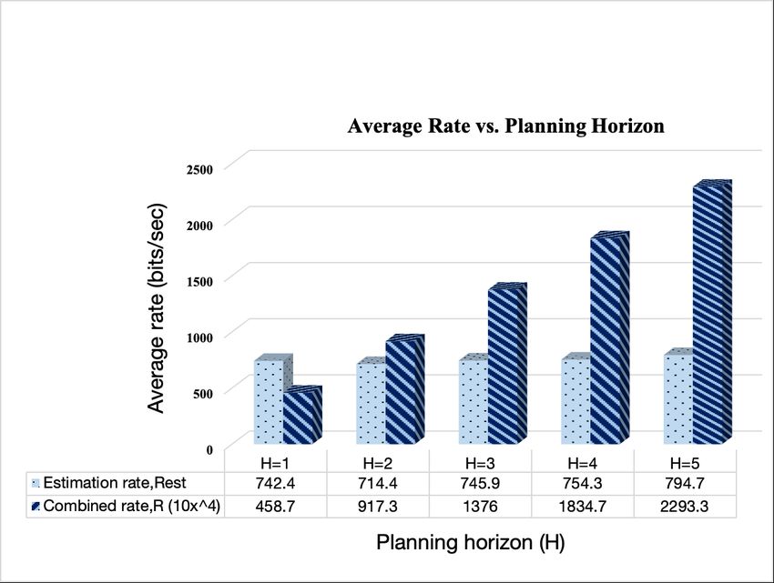
100 but at the same time the computational complexity in solving
10 7 Eq. 6 with H = 5 is significantly higher than with H = 1. In
0
0 0.1 0.2 0.3 0.4 0.5 0.6 0.7 0.8 0.9 fact, this computational complexity grows exponentially with
Blending parameter( ) H. Thus, one may need to assess if it is worth trading off
computational complexity for better performance, and then
Fig. 4: Average rate vs. α determine the planning horizon length H accordingly. Figure 6
shows the quantitative comparison of radar estimation rate
and average combined rate for five different planning horizon.
This trade-off property of the system is the reason we need to Figure 7 shows the qualitative comparison of planning horizon
optimize the waveform parameters over a planning horizon as H = 1 vs. H = 5. In both cases the size of the error
opposed to one-step optimization. We show a rate-rate curve confidence ellipse of the target increases when the target is
showing the communications and estimation rate for different occluded by the obstacles. But the size of the ellipse visibly
values of α where Rcomm is the SIC communications data reduces as we set H = 5. This reduction in the ellipse size
rate defined in Section III-A and α is a blending parameter is captured quantitatively in Figure 7. Table IV shows the
that is varied from 0 to 1. When α = 0, in Eq. 4 only
communications rate is considered, and when α = 1, only the
radar estimation rate is considered. In between, the product is
jointly maximized.
B. Impact of Planning Horizon on the Rates
In Figure 5, we plot the estimation rate for H = 1 and H =
5. At around time index 40, the line of sight is lost, which leads
to reduction in the estimation rate. As the line-of-sight gets
established at the time index 60, the rates go up in both cases,
but the rise is significantly higher for H = 5, which shows
that our non-myopic approach plans the waveform parameters
more effectively than the myopic approach (H = 1). Table III
summarizes the average combined rates for different planning
horizon lengths as discussed above. As we increase H = 1 to
H = 5 the combined rate is increased by more than five times, Fig. 6: Average rate vs. planning horizon
10
Authorized licensed use limited to: Tencent. Downloaded on June 30,2021 at 09:14:14 UTC from IEEE Xplore. Restrictions apply.Systems and Computers; Vol. 2018-October). IEEE Computer Society.
https://doi.org/10.1109/ACSSC.2018.8645080
[7] E. K. P. Chong, C. Kreucher, and A. O. Hero, “Partially observable
Markov decision process approximations for adaptive sensing,”Disc.
Event Dyn. Sys., vol. 19, pp. 377–422, 2009.
[8] S. Ragi and E. K. P. Chong, “UAV path planning in a dynamic envi-
ronment via partially observable Markov decision process,” IEEE Trans.
Aerosp. Electron. Syst.,vol. 49, pp. 2397–2412, 2013.
[9] A. Charlish and F. Hoffmann, “Anticipation in cognitive radar using
stochastic control,” in Proc. IEEE Radar Conf., Arlington, VA, 2016,
pp. 1692–1697.
[10] S. Ragi, E. K. P. Chong, and H. D. Mittelmann, “Mixed-integer nonlinear
(a) Planning Horizon H=1 (b) Planning Horizon H=5 programming formulation of a UAV path optimization problem,” in Proc.
2017 American Control Conf., Seattle, WA, 2017, pp. 406–411.
Fig. 7: Myopic vs. non-myopic approach [11] T. M. Cover and J. A. Thomas, Elements of Information Theory,2nd ed.
TABLE IV: Planing horizon length (H) Versus Average target Hoboken, New Jersey: John Wiley & Sons, 2006.
[12] A. R. Chiriyath, B. Paul, G. M. Jacyna, and D. W. Bliss, “Inner
location error bounds on performance of radar and communications co-existence,”IEEE
Transactions on Signal Processing, vol. 64, no. 2, pp. 464–474, January
Planing horizon length (H) Average target location error (m)
2016.
1 107.4344 [13] B. Paul and D. W. Bliss, “Extending joint radar-communications bounds
2 102.7342 for FMCW radar with Doppler estimation,” in IEEE Radar Conference,
3 94.9062 May 2015, pp. 89–94.
[14] B. Paul and D. W. Bliss, “The constant information radar,” En-
4 73.7049
tropy,vol. 18, no. 9, p. 338, 2016. [Online]. Available: http://www.mdpi.
com/1099-4300/18/9/338
impact of plan horizon length on the average target location [15] A. Chiriyath, S. Ragi, H. D. Mittelmann, D. W. Bliss, ”Novel Radar
Waveform Optimization for a Cooperative Radar-Communications Sys-
error. tem,”IEEE Transactions on Aerospace and Electronic Systems , vol. 55,
V. C ONCLUSIONS no. 3, pp. 1160–1173, April 2019.
[16] A. Chiriyath, S. Ragi, H. D. Mittelmann, D. W. Bliss, ”Radar Waveform
We developed a decision theoretic framework for adap- Optimization for Joint Radar Communications Performance,” Electronics,
tive waveform design in joint radar-communications systems. special issue on Cooperative Communications for Future Wireless Sys-
tems, vol. 8, no. 12, December 2019.
Specifically, we posed the waveform design problem as a [17] MATLAB’s fmincon. 2016. [Online]. Available: https://www. math-
partially observable Markov decision process (POMDP) and works.com/help/optim/ug/fmincon.
extended an approximated dynamic programming approach to [18] B. Paul, A. R. Chiriyath, and D. W. Bliss. Survey of rf communications
and sensing convergence research. IEEE Access, 5:252–270, 2017.
solve the problem in near real-time. Particularly, we adapted [19] S. Ragi and E. K. P. Chong, “Decentralized guidance control of UAVs
an ADP approach called nominal belief-state optimization with explicit optimization of communication,” J. Intell. Robot. Syst., vol.
or NBO. The goal is to optimize the spectral shape of the 73, pp. 811–822, 2014.
[20] A. R. Chiriyath and D. W. Bliss, “Joint radar-communications per-
radar waveform over time to maximize the joint performance formance bounds: Data versus estimation information rates,” in 2015
of radar and communications in spectral coexistence. We IEEE Military Communications Conference, MILCOM, October 2015, pp.
presented the quantitative benefits, in terms of communications 1491–1496.
[21] A. R. Chiriyath and D. W. Bliss, “Effect of clutter on joint radar-
and radar estimation rates, of our POMDP-based non-myopic communications system performance inner bounds,” in 2015 49th Asilo-
approach in waveform design against myopic or greedy ap- mar Conference on Signals, Systems and Computers, November 2015,
proaches. In our future studies, we will address challenges pp. 1379–1383.
[22] B. Paul, D. W. Bliss, and A. Papandreou-Suppappola, “Radar tracking
including time-varying communication demand and target waveform design in continuous space and optimization selection using
detection probability. differential evolution,” in 2014 48th Asilomar Conf. Signals, Systems and
R EFERENCES C ITED Computers, November 2014, pp. 2032–2036.
[23] J. R. Guerci, R. M. Guerci, A. Lackpour, and D. Moskowitz, “Joint
[1] J. B. Evans, “Shared Spectrum Access for Radar and Communica- design and operation of shared spectrum access for radar and communi-
tions (SSPARC),Online:http://www.darpa.mil/program/shared-spectrum- cations,” inIEEE Radar Conference, May 2015, pp. 761–766.
access-for-radar-and-communications. [24] M. Bica, K.-W. Huang, V. Koivunen, and U. Mitra, “Mutual information
[2] D. W. Bliss and S. Govindasamy, Adaptive Wireless Communications: based radar waveform design for joint radar and cellular communication
MIMO Channels and Networks. New York, New York: Cambridge systems,” in IEEE International Conference on Acoustics, Speech and
University Press, 2013. Signal Processing (ICASSP), March 2016, pp. 3671–3675.
[3] D. W. Bliss, “Cooperative radar and communications signaling: The [25] M. R. Bell, N. Devroye, D. Erricolo, T. Koduri, S. Rao, and D. Tuninetti,
estimation and information theory odd couple,” in Proc. IEEE Radar “Results on spectrum sharing between a radar and a communications sys-
Conference, May 2014, pp. 50–55. tem,” in 2014 International Conference on Electromagnetics in Advanced
[4] B. Paul, A. R. Chiriyath, and D. W. Bliss, “Joint communications and Applications (ICEAA), August 2014, pp. 826–829.
radar performance bounds under continuous waveform optimization: The [26] R. M. Gutierrez, A. Herschfelt, H. Yu, H. Lee, and D. W. Bliss. Joint
waveform awakens,” in IEEE Radar Conference, May 2016, pp. 865–870. radar-communications system implementation using software defined
[5] P. Chavali and A. Nehorai, “Cognitive radar for target tracking in mul- radios: Feasibility and results. In 2017 51st Asilomar Conference on
tipath scenarios,” in Proc. Waveform Diversity & Design Conf., Niagara Signals, Systems, and Computers, pages 1127–1132, Oct 2017.
Falls, Canada, 2010. [27] A. R. Chiriyath, B. Paul, and D. W. Bliss. Radar-communications
[6] Ma, O., Chiriyath, A. R., Herschfelt, A., & Bliss, D. (2019). Cooperative convergence: Coexistence, cooperation, and co-design.IEEE Transactions
Radar and Communications Coexistence Using Reinforcement Learning. on Cognitive Communications and Networking,3(1):1–12, March 2017.
In M. B. Matthews (Ed.), Conference Record of the 52nd Asilomar [28] B. Paul, C. D. Chapman, A. R. Chiriyath, and D. W. Bliss. Bridging
Conference on Signals, Systems and Computers, ACSSC 2018 (pp. 947- mixture model estimation and information bounds using i-mmse. IEEE
951). [8645080] (Conference Record - Asilomar Conference on Signals, Transactions on Signal Processing, 65(18):4821–4832,Sept. 2017.
11
Authorized licensed use limited to: Tencent. Downloaded on June 30,2021 at 09:14:14 UTC from IEEE Xplore. Restrictions apply.You can also read