Algebraic Ground Truth Inference: Non-Parametric Estimation of Sample Errors by AI Algorithms
←
→
Page content transcription
If your browser does not render page correctly, please read the page content below
Algebraic Ground Truth Inference: Non-Parametric
                                              Estimation of Sample Errors by AI Algorithms

                                                             Andrés Corrada-Emmanuel                            Edward Pantridge
                                                                    Data Engines                                    Swoop
                                                         andres.corrada@dataengines.com                          ed@swoop.com
arXiv:2006.08312v1 [stat.ML] 15 Jun 2020

                                                    Edward Zahrebelski                Aditya Chaganti                 Simeon Simeonov
                                                          Swoop                            Swoop                           Swoop
                                                     eddie@swoop.com                 aditya@swoop.com                  sim@swoop.com

                                                                                         Abstract

                                                    Binary classification is widely used in ML production systems. Monitoring classi-
                                                    fiers in a constrained event space is well known. However, real world production
                                                    systems often lack the ground truth these methods require. Privacy concerns may
                                                    also require that the ground truth needed to evaluate the classifiers cannot be made
                                                    available. In these autonomous settings, non-parametric estimators of performance
                                                    are an attractive solution. They do not require theoretical models about how the
                                                    classifiers made errors in any given sample. They just estimate how many errors
                                                    there are in a sample of an industrial or robotic datastream. We construct one such
                                                    non-parametric estimator of the sample errors for an ensemble of weak binary clas-
                                                    sifiers. Our approach uses algebraic geometry to reformulate the self-assessment
                                                    problem for ensembles of binary classifiers as an exact polynomial system. The
                                                    polynomial formulation can then be used to prove - as an algebraic geometry
                                                    algorithm - that no general solution to the self-assessment problem is possible.
                                                    However, specific solutions are possible in settings where the engineering context
                                                    puts the classifiers close to independent errors. The practical utility of the method
                                                    is illustrated on a real-world dataset from an online advertising campaign and a
                                                    sample of common classification benchmarks. The accuracy estimators in the
                                                    experiments where we have ground truth are better than one part in a hundred.
                                                    The online advertising campaign data, where we do not have ground truth data,
                                                    is verified by an internal consistency approach whose validity we conjecture as
                                                    an algebraic geometry theorem. We call this approach - algebraic ground truth
                                                    inference

                                           1   Introduction

                                           The problem of self-assessment is everywhere in science and technology. Here we consider the
                                           self-assessment problem for an ensemble of binary classifiers. Is it possible to create a non-parametric
                                           estimator for the ensemble errors when we do not have the ground truth for their decisions? Yes. The
                                           constructive algorithm we present uses ideas from algebraic statistics, data streaming algorithms and
                                           errror-correcting codes to compute an estimate for the ground truth statistics of the errors made by
                                           the classifiers on the given sample.
                                           It may seem strange that we could estimate, without any theory of how the classifiers made those
                                           errors, a statistic of the errors when we do not have the ground truth for their correctness of their
                                           decisions. It certainly runs counter to all previous published approaches (e.g. Raykar et al. [1], Liu

                                           Preprint. Under review.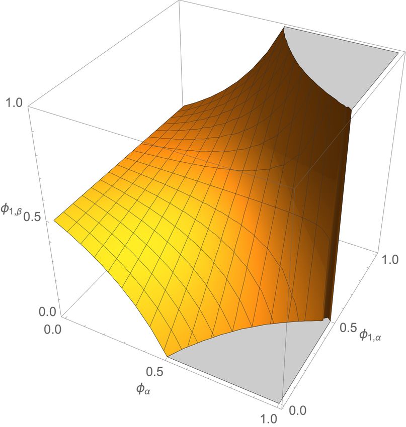
et al. [2], Zhou et al. [3], Zhang et al. [4]) to ground truth inference (GTI) - the estimation of sample
statistics that require the ground truth.

1.1   What is Ground Truth?

The term ground truth refers to the correct decisions the AI algorithm should have made on the given
sample. One could define the algebra presented here as being generally applicable to developing
self-assessment algorithms when one wants to estimate the error of noisy random estimators of
ground truth. In the case of binary classification, the ground truth is the correct label for each output
of the noisy estimator of the ground truth - the binary classifier.

1.2   Why estimation of ground truth statistics?

The motivation for GTI is simple and analogous to that used in data streaming algorithms. In
commercial or scientific settings, there is frequently one or two ground truth statistics that are
valuable. For example, speech recognition research and commercial development are mostly driven
by a single statistic of performance - Word Error Rate (WER). Similarly, when deploying binary
classifiers in an industrial AI pipeline, we can be satisfied with just knowing the average accuracy
of the classifiers. Therefore, we have observed that in many settings the role of curated data with
ground truth annotations is to carry out the correct calculation of a sample ground truth statistic. If so,
why not dispense with getting the ground truth and just estimate the wanted statistic?
This approach is also taken by data streaming algorithms like HyperLogLog. They forgo accumulating
the ground truth for the data and instead sketch it for the purposes of then estimating a wanted statistic.
In the case of HyperLogLog, it estimates the count of distinct values observed while refusing to
remember the ground truth for the data (the full set of distinct values so far observed).

1.3   The advantages and limitations of non-parametric estimation of AI errors

Taking a non-parametric approach to error estimation has many attractive features:

       • It bypasses the problem of understanding what model describes the way the classifiers are
         making errors. This means you do not need a meta-model of how the errors are being made.
       • It has a very small memory footprint. The binary classifier self-assessment sketch for three
         classifiers consists of eight integer counters.

Non-parametric estimation has one large theoretical disadvantage. No model of the data stream or
the performance of the binary classifiers is obtained. Having measured the error in a sample, we have
just that - a single number. There is no model to predict future or past errors. There is no model to
potentially assign causes to errors. Algebraic GTI only estimates the sample error. In that way it is no
different than other non-parametric estimators like HyperLogLog or Good-Turing smoothing.
Our approach to GTI differs from the previous literature on the subject. The concept that it is possible
to use an ensemble’s decisions to estimate each classifier’s error on the sample was first described
by Dawid and Skene [5]. The topic of GTI enjoyed a resurgence in the 2010s with many papers
[1, 6, 2–4] presented in NeurIPS and in other venues. An extensive 2017 survey by Zheng et al. [7]
of these approaches concluded that they were not stable across different domains. This is our main
critique of these methods - since they are Bayesian, they rely on carefully selected hyper-parameters
to estimate the uncertainty of the model they fit. But if we don’t have ground truth, how do we
know that a particular hyper-parameter setting is correctly capturing the errors in the sample? We do
not. The method presented here should be viewed, not as substitute for Bayesian models, but as a
complementary tool that can independently assess the errors on a given sample. The estimates of
algebraic GTI can then be used to guide a more appropriate hyper-parameter setting.
Another critique of Bayesian methods for self-assessment is that they will always return a best fit.
This is to be contrasted with the algebraic approach presented here where polynomial root solutions
may be outside the unit range or imaginary - a clear alarm that the assumptions inherent to the
approach are violated and cannot explain observed classifier decisions.

                                                    2
1.4 Algebraic methods for non-parametric estimation of AI errors
In the 1990s Pistone et al. [8] pioneered the use of algebraic geometry in statistics by recasting
traditional statistical tasks, such as experimental design, as polynomial problems.
The technique presented here also uses the math of algebraic geometry for a statistical task. Never-
theless, unlike previous Algebraic Statistics work, this technique is not concerned with models about
contingency table observations. Instead, it estimates true counts. Furthermore, there is no Algebraic
Statistics inside of Algebraic GTI, which is analogous to saying that Algebraic GTI can be used for
Algebraic Statistics but does not rely on Algebraic Statistics for the method to work.
2 Algebraic Geometry Of A Single Binary Classifier
Before tackling the full problem of an ensemble of binary classifiers, we discuss a simpler case - the
single classifier - to illustrate the language of algebraic geometry and how it relates to the problem of
self-assessment for a single classifier.
2.1 The polynomial system relating observable statistics to ground truth statistics
The black-box approach of non-parametric estimation means that the only observable sample statistic
for the classifier’s label decisions are the two counts, fα and fβ - the frequency of times the two
labels, α and β where observed in the sample. The sample values of these sample statistics are integer
ratios. Since these sample statistics are readily observed without needing knowledge of the ground
truth, we call them observables.
These point statistics are not the only ones possible for a given sample. For example, we may be
concerned with sequence statistics when reconstructing a DNA string. Thus our work here should not
be considered a general solution to any possible statistics for binary classifiers but as a solution for
the self-assessment problem for point statistics. In the Conclusion, we discuss the implications of this
for future research.
We write the two observable statistics for a single classifier in terms of the 5 unknown ground truth
statistics of this ensemble describing n = 1 as a polynomial system as follows,
fα = φα φ1,α,α + φβ φ1,β,α (1)
fβ = φα φ1,β,α + φβ φ1,β,β (2)
1 = fα + fβ (3)
1 = φ α + φβ (4)
1 = φ1,α,α + φ1,β,α (5)
1 = φ1,β,β + φ1,α,β . (6)
Here the φ1,`j ,`i variables are the unknown frequencies that classifier 1 identified `i as `j . The φα
and φβ variables are the unknown prevalences of the true labels in the sample. Ideally, we want to
solve for these statistics generally in terms of fα and fβ .
All the φ sample statistics fall into the 2nd category of sample statistics we call ground truth statistics.
These are sample statistics that require knowledge of ground truth to compute. With ground truth,
these sample statistics can be readily computed. The job of Algebraic GTI is to estimate these ground
truth statistics when they are missing.
Note, furthermore, that the ground truth statistics (the φ variables) are themselves divided into two
classes: the environmental ground truth statistics (the prevalence of the labels) and performance
ground truth statistics (the accuracy of the classifiers).
The polynomial system above can be simplified by eliminating some of the variables via the normal-
ization equations, which results in the following simpler polynomial system,
fα = φα φ1,α + (1 − φα )(1 − φ1,β ) (7)
fβ = φα (1 − φα,) + (1 − φα )φ1,β,β . (8)
Terms like φi,` represent the accuracy of the ith classifier on the ` label.
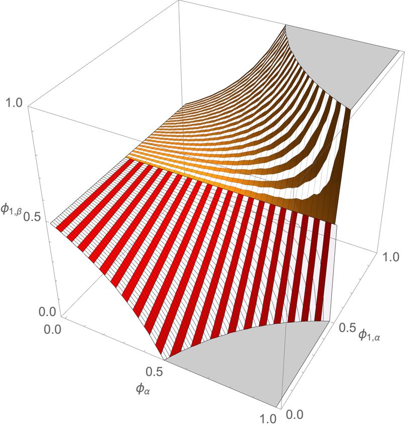
3(a) One classifier (b) Two classifiers (c) Three classfiers
Figure 1: The algebraic varieties for the self-assessment polynomials of varying numbers of classifiers
in the twonorm experiment. As more classifiers are added in the self-assessment, the uncertainty in
the ground truth statistics decreases to two points when three or more are used. Moving left to right,
the algebraic variety transforms from a surface in the single classifier case to a fractured surface in
the two classifier case and finally collapses into two individual points in the three classifier case.
Algebraic geometry is concerned with studying the geometric objects that correspond to zeros of a
polynomial system. The set of points in the polynomial variables space that satisfy these polynomials
is called an algebraic variety. In the case of one binary classifier that geometric object is a surface in
the three dimensional space of the (φα , φ1,α , φ1,β ) variables as shown in Figure 1(a).
Since the algebraic variety is a surface for one binary classifier, we conclude that a single binary
classifier cannot self-assess. The formal way to state this is as a property of the Gröbner basis for
equations 7 and 8 computed with the elimination order on monomials. Details are discussed in
Supplement A.
3 Algebraic Geometry of Self-Assessment for Two Binary Classifiers
We now consider an n = 2 ensemble of binary classifiers. Just like the case of n = 1, we can write
an exact polynomial description of the sample statistics. But having moved to using two binary
classifiers, we must account for non-independence between the errors made by each classifier within
a given sample.
While the formalism presented here can be extended to a classification of 3 or more labels by
using indicator functions, binary classification allows us to think of non-independence in terms of
covariance measures. In the case of two binary classifiers this requires that we introduce two new
ground truth statistics defined as follows,
S
1X
Γi,j,` = (xd,i − x̄i ) (xd,j − x̄j ) , (9)
S
d=1
where S is the size of the sample. The xd,i variables are 0/1 variables indicating whether the i
classifier correctly classified the item d in the sample. The x̄i variable is the average performance of
the classifier on the given label and sample. These happen to be identical to the φi,`,` statistics we are
trying to estimate.
We can now write the full, exact polynomial system for two binary classifiers,
fα,α = φα (φ1,α φ2,α + Γ1,2,α ) + (1 − φα ) ((1 − φ1,β )(1 − φ2,β ) + Γ1,2,β ) (10)
fα,β = φα (φ1,α (1 − φ2,α ) − Γ1,2,α ) + (1 − φα ) ((1 − φ1,β )φ2,β − Γ1,2,β ) (11)
fβ,α = φα ((1 − φ1,α )φ2,α − Γ1,2,α ) + (1 − φα ) (φ1,β (1 − φ2,β ) − Γ1,2,β ) (12)
fβ,β = φα ((1 − φ1,α )(1 − φ2,α ) + Γ1,2,α ) + (1 − φα ) (φ1,β φ2,β + Γ1,2,β ) . (13)
4It is important that the reader understand that this is not an approximate description of the self-
assessment problem for binary classifiers. If you had the sample values for all the variables on the
right of the equal signs in eqs 9-13 , these equations would evaluate to the exact values observed for
the left variables. This comes about because the sample statistics for the decisions of any number
of classifiers exist in a finite dimensional space. We can exhaustively enumerate all the sample
statistics - observables and ground truths statistics - that would explain the observed agreements
and disagreements between the classifiers. This is to be contrasted with any scientific model that
is seeking to explain the observed errors. Since we do not know what model would be correct, we
cannot know if our theory of why the errors occurred is underestimating or overestimating the correct
number of parameters. That model uncertainty does not exist when we just consider sample statistics
estimation and forego any further theoretical understanding of why the classifiers are making mistakes
on a data stream.
3.1 The two binary classifier self-asssessment problem is unsolvable
The self-assessment problem for two binary classifiers is also unsolvable in full generality. A naive
counting argument shows why. Since the observable frequencies must sum to one, there are really
only 3 independent equations in this case. But to obtain point solutions, we would have to solve for 7
variables. This result is also formalized in Supplement A as an Algebraic Geometry algorithm.
The estimation is also impossible even if the two binary classifiers were not correlated on the sample
(Γi,j,` = 0). In that case, we would have to solve for 5 ground truth statistics, but again fall short of
having only 3 independent equations. The unsolvability is illustrated in Figure 1(b) for one of the
classifiers in the n = 2 ensemble (classifier 1 of the twonorm experiment), the extra information of
comparing with the other classifier (classifier 2 in the twonorm experiment) divides the n = 1 surface
into two disjoint pieces. This unsolvability for independent binary classifiers changes dramatically
when we move on to consider the n = 3 case.
4 Algebraic Geometry of Self-Assessment for Three Binary Classifiers
Three independent binary classifiers can solve the self-assessment problem in certain circumstances.
Before we discuss the solution, let us consider again the issue of general unsolvability using possibly
sample-correlated classifiers. Once we move to three or more classifiers there is an explosion in the
number of variables needed to describe the non-independence between the classifiers. We can do a
full accounting of the dimension of that space.
• One environmental ground truth statistic, φα .
• Two performance ground truth statistics for the accuracies of each classifier, φi,α and φi,β .
• m ground truth statistics for the m-way correlation on each label. For 2-way correlations on
a label we would need n choose 2, and so on.
The number of variables (the dimension of the space) needed to describe all sample statistics of n
classifiers is,2n+1 − 1. This immediately makes it obvious that the general self-assessment solution
for n classifiers is impossible since the event space of the decisions of n of them would be 2n for
binary classification. The polynomial exact formulation is always short by about half the number of
variables we need to estimate.
If we were doing sequence ground truth statistics, instead of the point ground truth statistics treated
here, the dimension of the sample statistic space would be larger. But, in addition, there would be
an increase in the observable statistics and their corresponding polynomial equations. These more
complicated self-assessment polynomial systems are an area of future research.
4.1 The full solution for three independent binary classifiers
In spite of the general unsolvability of the self-assessment problem for binary classifiers, at n = 3 a
new phenomena arises. It is now possible to solve the GTI problem for independent binary classifiers.
5Table 1: Self-assessment runs on three Penn ML Benchmarks [10]
Benchmark Prevalence C1 C2 C3
twonorm 0.501(0.500) 0.887(0.884) 0.885(0.880) 0.863(0.864)
ring 0.574(0.505) 0.673(0.709) 0.602(0.703) 0.610(0.708)
mushroom 0.596(0.518) 0.948(0.814) 0.877(0.798) 0.732(0.782)
The polynomial system for three independent classifiers is,
fα,α,α = φα φ1,α φ2,α φ3,α + (1 − φα )(1 − φ1,β )(1 − φ2,β )(1 − φ3,β ) (14)
fα,α,β = φα φ1,α φ2,α (1 − φ3,α ) + (1 − φα )(1 − φ1,β )(1 − φ2,β )φ3,β (15)
fα,β,α = φα φ1,α (1 − φ2,α ) φ3,α + (1 − φα )(1 − φ1,β )φ2,β (1 − φ3,β ) (16)
fβ,α,α = φα (1 − φ1,α ) φ2,α φ3,α + (1 − φα )φ1,β (1 − φ2,β )(1 − φ3,β ) (17)
fβ,β,α = φα (1 − φ1,α ) (1 − φ2,α ) φ3,α + (1 − φα )φ1,β φ2,β (1 − φ3,β ) (18)
fβ,α,β = φα (1 − φ1,α ) φ2,α (1 − φ3,α ) + (1 − φα )φ1,β (1 − φ2,β )φ3,β (19)
fα,β,β = φα φ1,α (1 − φ2,α ) (1 − φ3,α ) + (1 − φα )(1 − φ1,β )φ2,β φ3,β (20)
fβ,β,β = φα (1 − φ1,α ) (1 − φ2,α ) (1 − φ3,α ) + (1 − φα )φ1,β φ2,β φ3,β . (21)
This polynomial system contains 7 unknown ground truth statistics, and there are 7 independent
equations. Any algebraic geometry computer system can solve this problem. In Mathematica, this
polynomial problem can be solved in about 5 seconds on a standard laptop. A full general solution
for the independent case is also possible by calculating the Gröbner basis with elimination order
for the monomials as mentioned before. This utilizes the Buchberger algorithm for computing a
Grobner basis for the ideal of the polynomial system[9]. For this system of polynomials, it returns
a sequence of polynomials with progressively fewer variables. The bottom one, involving only the
single φα variable is a quadratic. The coefficients of the quadratic are very complicated functions of
the f variables. One coefficient contains more than 1K terms. Nonetheless, when the f values are
plugged into the quadratic it is simply a quadratic polynomial on φα with integer ratio coefficients.
Therefore there could be be two real solutions with all values in the (0,1) range as required for the
ground truth integer ratios. We call roots that fall outside the (0,1) unphysical. Details are given in
Supplement A.
This ambiguity may seem to contradict our assertion that the self-assessment problem is solvable for
independent binary classifiers. In the right engineering context it is possible to remove the ambiguity
with side information. For example, this ambiguity of the "decoding" for self-assessment is entirely
analogous to the decoding ambiguity in error-correcting codes for detecting and correcting bit flips in
computers. There too, there is always more than one decoding solution. An error could be caused by
one bit flip or seven. What makes algebraic GTI practical is the same thing that makes error-correcting
codes practical. In the right engineering context, you may be assured that a majority of the classifiers
are better than random. Or the prevalence may be environmentally stable such as when detecting rare
items. In such a case, we would pick the solution that had the rare object at 1% of prevalence rather
than at 99%.
5 Self-Assessment Experiments in Three Standard Binary Classification
Benchmarks
We tested the practicality of estimating unknown binary classifier performance by searching the Penn
Machine Learning Benchmarks (PMLB) database [10] to see if any benchmark fulfills the conditions
that would allow us to treat the classifiers as independent. We found three benchmarks (twonorm,
ring, and mushroom)t hat had enough data and showed low correlation between the features used
for training. The results are summarized in Table 1.
Since the assumption of independence always creates two solutions, how could we decide which one
was correct for presentation in Table 1? Consider the twonorm experiment with 7,400 predictions.
The two solutions are shown in Table 2. We picked root solution 2 with the following reasoning:
In an engineering context of a well-designed set of classifiers, it is highly likely that the classifiers
perform better than random. Is it more likely that all three classifiers have failed or that all three are
6Table 2: The two self-assessment solutions for a single twonorm experiment
Root Solution Prevalence C1 C2 C3
1 0.499 0.117 0.119 0.133
2 0.501 0.887 0.885 0.863
Table 3: The mushroom benchmark failure on the β label accuracies, φi,β .
C1 C2 C3
1.001(0.916) 0.848(0.939) 0.868(0.742)
okay? This side information is entirely analogous to error-correcting codes picking a few bit flips
versus many bit flips when they decode an error-correcting code.
In contrast, the solution obtained for the mushroom benchmark is a failure for the independent
polynomial system. For consistency and ease of presentation, Table 1 shows only the accuracies for
the most common label in each benchmark. Let us call that φi,α . But the accuracies for the β label
returned a non-physical answer for the 1st classifier as detailed in Table 3.
The failure of mushroom should be noted as an actual strength of the algebraic approach. In actuality,
it returned non-sensical solutions. This is a clear alarm that the assumption of classifier independence
is violated in the mushroom experiment, which is detailed further in Supplement B.
6 Self-Assessment Experiments for Online ID Accuracy Systems
We now discuss a seemingly unrelated task which can, in fact, be mapped to a self-assessment
problem that is identical to the binary classifier polynomial system. We consider the problem of
measuring the accuracy of 4 different ID systems used in online advertising. This experiment is
important because, in fact, we do not have any knowledge of the true identities of the users who
were tagged with the noisy online anonymous IDs. So how could one be assured that a solution to
the independent classifier polynomial system is actually correct? The answer is very similar to the
approach of error-correcting codes.
In this experiment we have 4 noisy ID systems. Therefore, we can create 4 triplets that can then be self-
assessed with the 3 independent classifier polynomial estimator. Our claim is that the self-consistency
between the solutions obtained is that assurance. This can actually be stated as an algebraic geometry
conjecture. The resolution of the theorem remains an open problem (see Supplement C).
Online ID systems are not binary classifiers. They must produce an arbitrarily number of IDs that
could vary from context to context. However, we can take the stream of IDs produced by the ID
systems and map it into a binary stream by just asking from each ID system if it has observed the
ID before in the data stream. This creates a series of binary labels (new, old) that maps the problem
directly into the binary classifier polynomial system.
The results for the four triplet self-assessment solutions are shown in Table 4. The ambiguity of the
two solutions makes an automatic solution impossible. The engineering context in this case was
assumed to be that the majority of ID systems should be better than random on identifying new users.
The self-consistency between all possible triplet solutions is remarkable. Since the prevalence of
new users is precisely the unique count of entities under the ID systems, this algorithm is actually a
unique count estimator on data streams where we only have noisy Identity functions.
In addition, note that it can be implemented with a tiny memory footprint in comparison to algorithms
like HyperLogLog. This is, therefore, an example where noise actually decreases the memory
footprint of an algorithm. We discuss later on the implications of this observation for an alternative
architecture of artificial intelligence. Details of this experiment are discussed in Supplement C.
7Table 4: Comparing trio solutions for 4 ID systems
Triplet Unique Users % ID1 IP ID2 Swoop ID3 SR ID4 Vendor
(1,2,3) 0.797443 0.985041 0.999959 0.607004 N/A
(1,2,4) 0.799948 0.982922 0.999951 N/A 0.995661
(1,3,4) 0.795855 0.985627 N/A 0.607688 0.996777
(2,3,4) 0.799688 N/A 0.999984 0.605286 0.995952
7 Conclusions
A non-parametric error estimator of errors made by binary classifiers becomes possible when the
ensemble has three or more members. While a general solution to the self-assessment problem for
them is impossible, one can engineer classifiers that are close enough to independence to make this
method practical. We exhibited two Penn-ML benchmarks where the independent errors polynomial
system worked, and one where it failed. The failure is further indication of the utility of this non-
parametric approach since it signals to the user that the independent assumption is incorrect and
polynomial systems that include correlation parameters need to be used. Which contrasts with
Maximum Likelihood methods that will always return a best fit solution.
In addition, we discussed an experiment in an industrial setting where no ground truth is available for
the correct answers but the self-consistency of all possible trio solutions from 4 binarized outputs
strongly suggests the independence assumption was correct. An algebraic geometry conjecture that
will settle the question of whether the self-consistency can only be explained by independent errors
on the sample is discussed in Supplement C.
Broader Impact
Error is at the heart of Science. If you understand errors, you understand Science. Tools like algebraic
GTI can complement classifiers and regressors. We expect that new examples will be developed for
recommender systems, ranked lists, etc. Many other polynomial systems remain to be discovered
for the simple reason that while there is one ground truth, there are many statistics of ground truth.
We close with some questions about the possible significance of non-parametric estimators for
Neuroscience.
Is there an algorithm that can measure IQ without having any Psychology or World representation
inside of it? We do not know. But if the representation problem for intelligence gets one into circular
arguments, why not question the necessity of an assessor that has any intelligence? In this paper we
have discussed many algorithms that are able to monitor with the barest of theoretical assumptions.
The regression self-assessment solution by [11] could be used to monitor the signals from other cells.
If the brain is algorithmic, did it miss this whole class of algorithms?
The work here and in papers such as Corrada-Emmanuel and Schultz [11] have broad applications
for the safety engineering of AI systems. They allow a machine to self-assess its own performance.
As we have mentioned, while there is no general solution to the self-assessment problems discussed
here, in the right engineering context these solutions are practical and useful.
References
[1] Vikas C. Raykar, Shipeng Yu, Linda H. Zhao, Gerardo Hermosillo Valadez, Charles Florin, Luca Bogoni,
and Linda Moy. Learning from crowds. Journal of Machine Learning Research, 11(43):1297–1322, 2010.
[2] Qiang Liu, Jian Peng, and Alexander T Ihler. Variational inference for crowdsourcing. In F. Pereira, C. J. C.
Burges, L. Bottou, and K. Q. Weinberger, editors, Advances in Neural Information Processing Systems 25,
pages 692–700. Curran Associates, Inc., 2012.
[3] Dengyong Zhou, Sumit Basu, Yi Mao, and John C. Platt. Learning from the wisdom of crowds by minimax
entropy. In F. Pereira, C. J. C. Burges, L. Bottou, and K. Q. Weinberger, editors, Advances in Neural
Information Processing Systems 25, pages 2195–2203. Curran Associates, Inc., 2012.
8[4] Yuchen Zhang, Xi Chen, Dengyong Zhou, and Michael I Jordan. Spectral methods meet em: A provably
optimal algorithm for crowdsourcing. In Z. Ghahramani, M. Welling, C. Cortes, N. D. Lawrence, and K. Q.
Weinberger, editors, Advances in Neural Information Processing Systems 27, pages 1260–1268. Curran
Associates, Inc., 2014.
[5] P. Dawid and A. M. Skene. Maximum likelihood estimation of observer error-rates using the em algorithm.
Applied Statistics, pages 20–28, 1979.
[6] Fabian L Wauthier and Michael I. Jordan. Bayesian bias mitigation for crowdsourcing. In J. Shawe-Taylor,
R. S. Zemel, P. L. Bartlett, F. Pereira, and K. Q. Weinberger, editors, Advances in Neural Information
Processing Systems 24, pages 1800–1808. Curran Associates, Inc., 2011.
[7] Y. Zheng, G. Li, Y. Li, C. Shan, and R. Cheng. Truth inference in crowdsourcing: Is the problem solved?
In Proceedings of the VLDB Endowment, volume 10, no. 5, 2017.
[8] G. Pistone, E Riccomagno, and H. P. Wynn. Algebraic Statistics: Computational Commutative Algebra in
Statistics. Chapman and Hall, 2001.
[9] D. Cox, J. Little, and D. O’Shea. Ideals, Varieties, and Algorithms: An Introduction to Computational
Algebraic Geometry and Commutative Algebra. Springer-Verlag, 2015.
[10] Randal S. Olson, William La Cava, Patryk Orzechowski, Ryan J. Urbanowicz, and Jason H. Moore. Pmlb:
a large benchmark suite for machine learning evaluation and comparison. BioData Mining, 10(1):36,
Dec 2017. ISSN 1756-0381. doi: 10.1186/s13040-017-0154-4. URL https://doi.org/10.1186/
s13040-017-0154-4.
[11] A. Corrada-Emmanuel and Howard Schultz. Geometric precision errors in low-level computer vision tasks.
In Proceedings of the 25th International Conference on Machine Learning (ICML 2008), pages 168–175,
Helsinki, Finland, 2008.
9You can also read