High Cadence Optical Transient Searches using Drift Scan Imaging III: Development of an Inexpensive Drive Control System and Characterisation and ...
←
→
Page content transcription
If your browser does not render page correctly, please read the page content below
Publications of the Astronomical Society of Australia (PASA)
                                               doi: 10.1017/pas.2021.xxx.

                                               High Cadence Optical Transient Searches using Drift
                                               Scan Imaging III: Development of an Inexpensive Drive
                                               Control System and Characterisation and Correction of
                                               Drive System Periodic Errors
arXiv:2106.09406v1 [astro-ph.IM] 17 Jun 2021

                                               Steven Tingay
                                               International Centre for Radio Astronomy Research, Curtin University, Bentley, WA 6102, Australia

                                               Abstract
                                               In order to further develop and implement novel drift scan imaging experiments to undertake wide field,
                                               high time resolution surveys for millisecond optical transients, an appropriate telescope drive system
                                               is required. This paper describes the development of a simple and inexpensive hardware and software
                                               system to monitor, characterise, and correct the primary category of telescope drive errors, periodic
                                               errors due to imperfections in the drive and gear chain. A model for the periodic errors is generated
                                               from direct measurements of the telescope drive shaft rotation, verified by comparison to astronomical
                                               measurements of the periodic errors. The predictive model is generated and applied in real-time in
                                               the form of corrections to the drive rate. A demonstration of the system shows that that inherent
                                               periodic errors of peak-to-peak amplitude ∼10000 are reduced to below the seeing limit of ∼300 . This
                                               demonstration allowed an estimate of the uncertainties on the transient sensitivity timescales of the
                                               prototype survey of Tingay & Joubert (2021), with the nominal timescale sensitivity of 21 ms revised
                                               to be in the range of 20 − 22 ms, which does not significantly affect the results of the experiment. The
                                               correction system will be adopted into the final version of high cadence imaging experiment, which is
                                               currently under construction. The correction system is inexpensive (
2

cadence imaging technique depends on higher than side-          performance of the system are described. In Section 4
real rate tracking to achieve high time resolution, knowl-      the results are described and discussed, including an
edge of and control of the drive rates is very important.       estimate of uncertainties for the experiment described
Telescope drive systems of various levels of complexity         in Paper II. Finally, in Section 5, conclusions and future
require different levels of pointing corrections. At the        work is briefly described.
professional end, highly complicated models are required
to correctly point and track a large telescope (Hovey,
                                                                2 HARDWARE UNDER DEVELOPMENT
1974). At the amateur commercial end, many relatively
                                                                  AND TEST
inexpensive modern telescopes include a Periodic Error
Compensation (PEC) system (Saunders, 2012).                     A simple system has been chosen, based on very in-
   For the work under consideration here, which deals           expensive off-the-shelf parts available at any hobbyist
with optical systems of moderate size and is highly             electronics store and openly available software libraries
focused on the exploitation of inexpensive commercial-          for standard computing platforms.
off-the-shelf (COTS) equipment, periodic errors in the             The drive motor is driven and monitored via an
drive system (motor and gear trains) are the dominant           Arduino-based system, in order to measure periodic
form of error. Periodic errors are generally caused by          errors and feed corrections back to the drive system.
imperfections of various types in the manufacture and           The detected and corrected periodic errors are indepen-
meshing of the gear trains that transfer the motion of a        dently verified via direct astronomical measurements,
motor to the rotation of the telescope right ascension axis.    again using simple hardware.
The broad effect is the periodic speed-up and slow-down
of the motion of the telescope, relative to the sidereal
rate, causing an astronomical object to wander back             2.1 Optical assembly, mount, and camera
and forth on a sensor, in an east-west (right ascension)        The classic method of measuring periodic error in as-
direction. For the high cadence imaging application, the        tronomical telescope systems is via direct astronomical
effect will cause a variable transient sensitivity timescale.   measurements (Saunders, 2012). At the end of the day,
This should be understood and, ideally, corrected in the        this is the measurement that matters, the drift of the
drive system.                                                   position of an astronomical object across the sensor, as
   The goal of the work described here is to develop,           a function of time. Thus, these measurements are the
test, and demonstrate a simple and inexpensive system           ultimate source of verification for any periodic error
to characterise and correct periodic errors in the drive        correction system.
systems that will be used for the high cadence imaging             A simple optical assembly is used, a Skywatcher
application. A system of hardware and software, based           130mm aperture, 1000mm focal length reflector. With a
on the popular low cost Arduino platform and python             spherical primary and a catadioptric corrector before the
code, is developed that allows periodic errors to be mea-       secondary, the off-axis imaging quality is poor. But for
sured and characterised, independently of astronomical          a substantial on-axis area, stellar images are point-like
characterisation. The measurements are verified by astro-       and easily adequate for the measurement of periodic
nomical observations and are used to create a predictive        errors.
model for the correction of periodic errors.
                                                                   As the Canon RP full-frame sensor camera was se-
   This system is developed using the mount and drive           lected for the final high cadence imaging system, this
components used in Paper II, which allows an estimate           camera was utilised here, in order to gain general experi-
of the uncertainties due to periodic errors that affected       ence with it. The Canon RP was mounted to the optical
the experiment described in that paper. The system              assembly (with x and y sensor axes aligned north-south
is also developed in order to be adapted to the final           and east-west, respectively) and produced good results.
high cadence imaging instrument currently under con-            The sensor pixel size of 5.75µm corresponds to 100 .18
struction. In addition, this work utilises other hardware       with the optical assembly (on-axis). The camera was
components selected for the final system, such as the           controlled via a MacBook Pro laptop, running the Canon
Canon RP cameras, allowing experience to be gained              EOS Utility (version 3)1 .
with those components.
   The hardware and software system could be read-
ily adapted to many other situations, so design and             2.2 Arduino-based drive control and
construction details are provided here and all codes                measurement
are available at https://github.com/steven-tingay/High-
                                                                The telescope mount drive motor is a Nippon Pulse
Cadence-Imaging-III.
                                                                Motor Company PF42-48f3g stepper motor2 with 48
   In Section 2 the hardware components of the sys-
tem are described. In Section 3, the measurements and             1 hk.canon/en/support/0200593702

astronomical observations used to test and verify the             2 www.dynetics.eu/CMS/Docs/NPM/NPM     stepper cat.pdf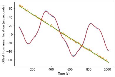
High Cadence Optical Transient Searches 3
steps/revolution and a 200:1 gearhead, giving 0.0375 A schematic wiring diagram for the motor, Uno, Servo
deg/step. The further gear reduction of 180:1 provided Controller Module, RTC, and rotary encoder is provided
by the worm and worm gear assembly of the mount in Figure 1. All of the Arduino components cost, in total,
gives 0.00 75/step driving of the right ascension axis of the less than $A100.
mount. The nominal sidereal tracking rate corresponds
to one rotation of the worm every 8 minutes, which in
turn corresponds to a rotation rate of the motor of 25
RPM.
The PF42-48f3g motor is a bipolar stepper with the
rotor driven by two coils, with two leadwires per coil,
which connect to an Arduino Uno (Rev 3) board 3 and
an Arduino Compatible Motor Servo Controller Module4 .
Control of the motor was then enabled by writing an
Arduino sketch based on the AFMotor library5 and
supporting python3 scripts. All code for this work is
available from https://github.com/steven-tingay/High-
Cadence-Imaging-III.
In order to have access to accurate timing information,
a Real Time Clock (RTC) module6 was connected to
the Arduino board. The RTC was accessed in the sketch
via the DS1307RTC libray 7 and the Time library8 .
Finally, in order to make direct measurements of the
periodic errors in the system, a rotary encoder was at-
tached to the worm shaft and connected to the Arduino
board. The rotary encoder utilised is a quadrature en-
coded 20 step digital encoder9 . The quadrature encoding
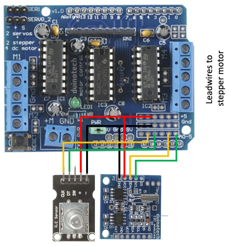
Figure 1. The schematic wiring diagram for the Arduino-based
is generally utilised to sense the direction of rotation. drive monitor/controller, showing the motor servo controler board
However, at low rotation speeds (such as the 8 minute (which mates to the top of an Arduino Uno board), the rotary
period of the worm), the quadrature encoding can be encoder (bottom left), and the real time clock (bottom right). The
conveniently used to detect four sub-steps between each port that connects to the stepper motor is indicated, but wiring is
not shown, as this will be dependent on the motor selected. The
digital step. Thus, the rotary encoder produces 80 sub- quadrature encoded signals from the rotary encoder are carried
steps per rotation, corresponding to 4.5 degree steps of on pins CLK and DT. If these signals are unreliably read, the
the worm and, due to the 180:1 gear reduction of the addition of a 100 nF capacitor between each these pins and GND
worm and worm gear assembly, 9000 increments in right will generally alleviate this issue. A 9V power connection to the
Uno and the USB connection to the laptop on the Uno are not
ascension. No special libraries are required to access the shown.
rotary encoder data, as the quadrature encoded mea-
surements are simply read on two of the Uno digital pins
using standard methods.
The sketch is loaded to the Uno from a MacBook Pro
laptop. The RTC is synchronised to laptop time at each 3 MEASUREMENTS AND DATA
execution of the sketch. Due to memory and processing PROCESSING
limitations on the Uno board itself, data collected by
3.1 Astronomical measurements
the Uno are processed both on the Uno and the laptop.
Data and processing results are passed back and forth The most direct measurement of periodic error in a
between the Uno and the laptop via a python3 script, telescope system comes from astronomical measurements.
utilising the pyserial library10 . Thus, as a mechanism to understand the magnitude of
3 store.arduino.cc/usa/arduino-uno-rev3 the errors that the correction system needs to address,
4 www.jaycar.com.au/medias/sys_master/images/ these measurements were undertaken first.
images/9505700151326/XC4472-manualMain.pdf Utilising the mount and camera system described
5 learn.adafruit.com/afmotor-library-reference/af-stepper-
above, and running the Arduino-based motor control
class
6 www.jaycar.com.au/medias/sys_master/images/ system for nominal sidereal tracking, a bright star was
images/9485758693406/XC4450-manualMain.pdf acquired on-axis and at the centre of the camera sensor.
7 www.arduino.cc/reference/en/libraries/ds1307rtc/
8 www.arduino.cc/reference/en/libraries/time/
Over two rotations of the worm, corresponding to
9 www.jaycar.com.au/medias/sys_master/images/ 16 minutes, images of one second exposure length were
images/9506700066846/XC3736-manualMain.pdf obtained every five seconds, resulting in 192 images over
10 pypi.org/project/pyserial/ the 16 minutes.4
The bright star was the brightest object in the field-of- R = rR t + oR + a sin (bt + c)+
view, thus a simple python script (pe.py; included in the + d sin (et + f ) + g sin (ht + i) (2)
github repository for the project) was developed to detect
the star in each image and record its sensor location where: D is the position on the sensor in the declina-
in pixel coordinates (converted to relative arcseconds), tion direction (x-axis), in arcseconds; rD is the linear
along with the time of measurement. drift rate in the declination direction, in arcseconds per
The script uses the rawpy11 python module to read second; oD is the offset in the declination direction in
the Canon CR3 RAW format images, demosiac them arcseconds. This describes a linear drift in the north-
to produce images in the R, G, and B channels cor- south direction. Also, R is the position on the sensor in
responding to the Bayer filter (interpolating over the the right ascension direction (y-axis), in arcseconds; rR
missing pixel values for each colour), and combine the is the linear drift rate in the right ascension direction
normalised R, G, and B images into a grayscale image. in arcseconds per second; oR is the offset in the right
Thus, every pixel in the grayscale image is the result of ascension direction in arcseconds; a, d, and g are the am-
one measured value and two interpolated values, which plitudes of three sinusoidal periodic errors, in arcseconds;
means the physical pixel resolution (5.75µm ∼ 1.00 2) can b, e, and h are the corresponding angular frequencies of
be used in the analysis. the the three sinusoids i radians per seconds, 2π T , where
From the greyscale images, the coordinates of the T is the sinusoid period in seconds; and c, f , and i
pixel with the peak value in each image is recorded are the corresponding sinusoid phase offsets, in radians.
and utilised as the estimated position of the star as a This describes a linear drift with three superimposed
function of time. sinusoids in the east-west direction.
A typical example of the results obtained from these Figure 2 shows that these functions for the north-south
measurements can be seen in Figure 2, where the top and east-west motions describe the data very well. As
panel shows the drift of the star in the north-south and expected, the highest amplitude sinusoid has an angular
east-west directions and the bottom panel shows the frequency corresponding to the nominal 8 minute worm
(x,y) sensor domain drift as functions of time. rotation period. The other two sinusoid periods appear
The north-south drift is seen as linear with time, at twice and four times the primary angular frequency.
resulting from a very small misalignment of the mount Table 2 lists the fit parameters corresponding to the data
with true north. This is not a concern and is easily in Figure 2. Over many tests, the angular frequencies
addressed with a small correction to the mount. However, were very consistent and were thus fixed in all subsequent
the drift is advantageous as it makes it easy to inspect fitting of data, at 0.0131 rad/s, 0.0262 rad/s, and 0.0524
what is going on in the east-west direction, which is of rad/s, respectively.
primary interest as the direction affected by periodic
errors. 3.2 Drive shaft encoder measurements
In the east-west direction, a small linear drift can
be seen over time, corresponding to a small error in The rotary encoder attached to the worm shaft is in-
the nominal sidereal rate of the drive, superimposed tended to directly measure any variations in the rotation
with a large amplitude periodic error, with peak-to-peak of the worm that drives the worm gear attached to the
variation of approximately 80 − 100 arcseconds and right ascension axis. The intent of these measurements is
period close to the 8 minute period of the worm. A to find an empirical relationship between the worm shaft
random jitter in position due to seeing, of approximately phase and the motion of the star on the sensor, in an
3 − 5 arcseconds, is also apparent. This is largely what east-west direction. If a relationship is found, the rotary
is expected from a drive system of this quality and the encoder data can be used to predict corrections to the
observing location (same as for Papers I and II). drive motor, without further reference to astronomical
While of large amplitude, the periodic errors are data.
smooth and repeatable over a worm rotation. Inspection As the rotary encoder only measures the phase of the
also hints at multiple periodic error components. In order shaft as a function of time (with an arbitrary phase
to characterise both north-south and east-west motions, offset), the measurement captures the combined effects
guided by the visual inspection, python code using the of all elements in the gear chain, including the gearhead
scipy curvefit module12 was used to fit functions to these in the stepper motor, the worm, and worm gear (in so
motions, as follows: far as it affects the worm). An analysis to isolate the
individual periodic errors in each transmission element
is well beyond the scope of this work and this is not
D = rD t + oD (1) attempted. Only the empirical aggregate effect of the
11 https://pypi.org/project/rawpy/ periodic errors is considered.
12 https://docs.scipy.org/doc/scipy/reference/generated/ A typical example of the rotary encoder data is shown
scipy.optimize.curve_fit.html in Figure 3, corresponding to the same observation pe-High Cadence Optical Transient Searches 5
Table 1 Parameters for fit to north-south and east-west motion astronomical measurements
rD oD rR oR a/d/g b/e/h c/f /i
00 00 00 00 00
/s /s rad/s rad
−0.139 3889 −0.059 2673 41.5/−4.2/4.6 0.013/0.052/0.026 2.82/−5.80/−7.06
encoder; rP is the linear rate of the rotary encoder in
steps per second; oP is an arbitrary offset in steps (upon
every restart of the sketch, the step phase is set to zero);
j, m, and q are the sinusoid amplitudes, in steps; k, n,
and s are the corresponding sinusoid angular frequencies
in radians per second, fixed at values of k = 0.0131,
n = 0.0524, and s = 0.0262, as noted above; and l, p,
and u are the corresponding sinusoid phase offsets in
radians. Table 3 gives the fitted parameters, similar to
those given for the astronomical data in Table 2, and
the function is shown in Figure 3.
Figure 3. The phase of the worm shaft, as measured with the
Figure 2. Top panel: The drift of the star on the sensor in the
rotary encoder, with vertical axis in units of the encoder steps,
north-south (x-axis) direction (orange points and green linear
over the same period as the astronomical data shown in Figure
fit) and in the east-west (y-axis) direction (blue points and red
2. Data are shown in blue, the fitted model from Equation 3 is
sinusoidal fit), as described in the text. Bottom panel: Motion of
shown in orange.
the star on the sensor in the (x,y) domain. The motion starts at
the green marker and the motion ends at the red marker.
Care was taken to ensure that the sense of rotation
measured by the rotary encoder matched the sense of
riod as the astronomical data shown in Figure 2, after the motions on the sensor measured astronomically, so
the sidereal tracking rate has been removed from the that the two datasets could be compared and examined
data. Similar to the astronomical data, a periodic error to determine the relationship between them.
with angular frequency corresponding to the 8 minute
worm period is evident. While the data appear noisier
than the astronomical data, due to the fact that the 4 RESULTS AND DISCUSSION
encoder allows only 80 steps per worm period, some
In order to compare the data collected from the rotary
evidence of multiple periods are present in the data.
encoder and the astronomical measurements, the rotary
An identical approach to fitting the astronomical data
encoder units of steps need to be converted into the
was adopted for the rotary encoder data, as follows:
astronomical measurement units of arcseconds. This is
expressed as:
P = rP t + oP + j sin (kt + l)+
1.296 × 10⁶ Psteps
+ m sin (nt + p) + q sin (st + u) (3) Parcsec = (4)
SG
where the parameters are described by analogy to where: P(arcsec is the displacement on the sky in arcsec-
those in Equation 2. P is the phase in steps of the rotary onds caused by Psteps of the rotary encoder; 1.296 × 1066
Table 2 Parameters for fit to rotary encoder measurements
rP oP j/m/q k/n/s l/p/u
steps/s steps steps rad/s rad
−0.166 6.783 −0.483/0.036/0.097 0.0131/0.0524/0.0262 0.716/0.225/0.654
is the number of arcseconds in 360 degrees; S is the
number of steps per rotation of the rotary encoder (80
in this case); and G is the gear ratio of the worm and
worm gear assembly (180:1 in this case).
If this conversion is applied to the data in Figure 3
and compared to the data in Figure 2, Figure 4 results.
In this case, the data and the fit of the data for the
rotary encoder have been de-trended for the sidereal
rate and have both had the east-west drift rate derived
from the astronomical data applied, to provide ease of
visual comparison.
Figure 5. The rotary encoder measurements (red), fitted model
for the rotary encoder data (red line), model for the astronomical
measurements (blue line), and the difference between the rotary
encoder model and the astronomical model (green line), as a
function of time for an 8 minute period corresponding to one
worm rotation. The rotary encoder measurements and model have
been shifted by the 80 second offset from the astronomical model.
diction from the rotary encoder and the astronomical
measurements, which represents an expectation for how
well the periodic errors can be corrected. From an un-
Figure 4. The astronomical measurements of the periodic error,
corrected peak-to-peak amplitude of approximately 100
shown in black, with the fitted model of Equation 2 shown in arcseconds, the corrected data should be able to achieve
yellow. The rotary encoder data, shown in blue, with the fitted a peak-to-peak amplitude of approximately 10 arcsec-
model according to Equation 3 in orange, after conversion to onds.
astronomical units via Equation 4, is also shown.
The realisation of these corrections is dependent on a
data processing scheme that performs the rotary encoder
A good match of the rotary encoder data and the as- measurements, fits the three sinusoids to the rotary
tronomical data is evident, with a phase offset between encoder data, and then derives corrections from these fits
the two datasets. To examine the offset, both datasets and applies them to the drive motor rate, to compensate
were de-trended of any linear drift in the east-west direc- for the periodic errors.
tion and only the periodic errors were considered. Using This is achieved via the Arduino sketch and a python
the correlate function in the python numpy module, the script that collects and processes the rotary encoder
offset was determined to be 80 seconds. With this offset data, derives the corrections, and then controls the drive
removed, Figure 5 shows the comparison between both motor appropriately. Certain limitations on the levels of
datasets and both functional fits to the data, over a processing possible on the board, and limitations of the
single 8 minute rotation of the worm. various libraries utilised had to be overcome.
Figure 5 confirms an excellent match between a predic- For example, the Arduino Uno only has 2048 bytes of
tion based on the rotary encoder data and the measured on-board storage for code and variables. Thus, collections
astronomical effects, with an 80 second timing offset. of rotary encoder data are passed to the laptop via serial
Over many tests and trials, the 80 second offset is ro- communications, where the functional fit is performed.
bustly repeatable (with variations of ±2 seconds), but The fit parameters are sent back to the Uno board, where
the origin of the timing offset is unknown within the they are utilised to derive rate corrections for the drive
overall system of gears. motor, from the time derivative of Equation 3 along
Figure 5 also shows the difference between the pre- with the known time offset, as follows:High Cadence Optical Transient Searches 7
dPPE
= jk cos (k(t − toff ) + l)+
dt
+ mn cos (n(t − toff ) + p)+
+ qs cos (s(t − toff ) + u) (5)
The linear east-west drift term is omitted from the
correction (PPE only describes the periodic error com-
ponent), as it is separately dealt with as a constant
factor in the Arduino sketch, which also depends on
other aspects of the code implementation, such as the
adjustments required to maintain a constant update
period for the corrections. The corrections in Equation
5 only deal with the periodic error component.
An issue with the motor control library is that the
motor can only be controlled in integer values of RPM.
The drive rate variation required for this application
is generally in the range 23 to 27 RPM (centred on
the sidereal rate of 25 RPM) and requires smooth ad-
justment. A scheme by which the motor drive rate is
updated once every second at an integer rate is adopted,
with the residual between the exact required rate and
the integer rate added to the exact required rate for the
next update second, works well, but adds complexity
to the code. In order to maintain a one second update Figure 6. The results of verification tests of the periodic error
period, a variable number of stepper motor steps per correction process and software. The top panel shows the results of
a 960 calibration period and a further 960 second period when the
update is calculated, according to the integer RPM in derived corrections are applied, as seen in astronomical measure-
utilisation for that step. ments. The bottom panel shows an identical test at a later point
In this way, the overall sidereal tracking rate is main- in time, but with only half of the amplitude of the quarter period
tained with a regular update rate, modulated by the rate component of the correction applied, giving a superior result to
the top panel.
change corrections predicted by the rotary encoder data.
The many details of the codes are best described in the
comments included in the codes themselves, available
via the github repository at https://github.com/steven-
tingay/High-Cadence-Imaging-III. However, following the application of the corrections,
The periodic error correction scheme, and the code, even though the periodic errors are greatly reduced, some
was tested as follows. The hardware was setup as de- low level periodicity remains apparent after correction.
scribed above. A bright star was acquired and tracked The angular frequency of this residual periodic error
over a 1920 second period, corresponding to four rota- matches the fitted component at one quarter the period
tions of the worm. Upon execution of the sketch and of the worm. Thus, the test observations were re-run
the python code, the collection of 960 seconds of rotary with the application of only half the amplitude of this
encoder data was commenced. At the same time, the sinusoid component applied via the corrections. The
collection of 1920 seconds of images was commenced result is seen on the bottom panel of Figure 6, where
via the optical assembly and camera. At the end of the it is apparent that the residual periodic error has been
first 960 seconds, the model derived from the rotary removed. The RMS around the line of best fit in the
encoder data was transmitted to the Arduino board and period when corrections are applied is 300 .3, which is
thereafter the board generated drive rate corrections consistent with the seeing from the observing location
from the model and delivered them to the motor. and larger than the uncertainty due to the pixel size
Thus, the astronomical measurements cover the first of 1.00 2. Why this reduction in the amplitude of this
960 seconds (uncorrected periodic errors) and the second component of the correction is beneficial is not clear,
960 seconds (corrected periodic errors). The top panel but may be due to the coarse nature of the rotary encoder
of Figure 6 shows the results of this test, in the (x,y) steps emphasising variability at this angular frequency.
domain, confirming that the peak-to-peak amplitude It is possible that further investigation and trial and
in the east-west direction is reduced to the expected error may uncover the reasons for this improvement, or
approximate 10 arcseconds. allow refinements to this technique. For example, using8
more than two worm periods to derive the corrections and software and python code, the correction of periodic
will likely make the corrections more accurate. And errors to below the seeing limit is demonstrated for the
improving the timing of the system (both camera and drive system used in Paper II, allowing an estimate of
rotary encoder times are only good to approximately one the transient sensitivity timescales for that experiment;
second) may help improve the corrections. Finally, in rather than the quoted 21 ms timescales, a range of 20
Figure 6 the slow drifts in the north-south and east-west - 22 ms is strictly applicable to that experiment. The
directions have not been rectified, as they represent only conclusions of Paper II are not significantly affected.
very small mechanical adjustments to the mount and The periodic error correction system will be adapted
very small adjustments to the nominal sidereal tracking for the final version of the high cadence imaging experi-
rate in software, respectively. However, the bottom panel ment, which is currently under construction and due for
of Figure 6 shows that the corrections are now very close commissioning in the second half of 2021.
to seeing limited. Thus, the objective of the exercise, to The hardware and software developed for this pur-
obtain an empirical correction of the periodic errors, has pose can be readily adapted for a range of similar ap-
been achieved. plications, so the design details are provided. All codes
utilised for the system are also available in a github
repositary at https://github.com/steven-tingay/High-
4.1 Tracking uncertainties for published
Cadence-Imaging-III. While all hardware components
results
selected for this project are inexpensive, the methods
One motivation for undertaking this work was to quan- and codes can be adapted for different and/or higher
tify in detail the tracking errors relating to previously quality hardware components, for example higher quality
published work in Papers I and II. In particular, Paper rotary encoders with many more than 80 steps.
II published the first scientific results from the drift scan
imaging technique, to place constraints on the event
6 ACKNOWLEDGEMENTS
rate of optical transients with V magnitude less than
6.6. The quoted transient duration the experiment was This research has made use of NASA’s Astrophysics Data
sensitive to was 21 ms. System.
This sensitivity timescale was derived from the rate
of the sky motion across the pixels of the sensor, when
REFERENCES
driving the mount at four times the sidereal rate in the
anti-sidereal direction. Clearly, variations in the drive Arimatsu K., Tsumura K., Usui F., Ootsubo T., Watan-
rate can affect this timescale. abe J.-i., 2021, AJ, 161, 135
As the mount and motor used here was also used Burke-Spolaor S., 2018, Nature Astronomy, 2, 845
in Paper II, these effects can be quantified. The drive Hovey G. R., 1974, PhD thesis, Australian National
variations experienced in Paper II are exactly those University
shown in Figure 2 and tabulated in Table 2. Using the Richmond M. W., et al., 2020, PASJ, 72, 3
derivative of Equation 2 (similar to Equation 5) and the Saunders R., 2012, JRASC, 106, 162
coefficients from Table 2, the maximum variation from Tingay S., 2020, PASA, 37, e015
the sidereal rate can be calculated as 0.00 9 per second, Tingay S., Joubert W., 2021, PASA, 38, e001
corresponding to 6% of the sidereal rate.
Thus, the 21 ms quoted timescales in Paper II can be
up to 1 ms in error, when the periodic error gradient is
highest. For the vast majority of the time, the timescale
errors are significantly less than 1 ms. Therefore, the
results presented in Paper II are not significantly affected,
with the upper limits on the events rates now strictly
described as for transients in the range of 20 - 22 ms,
rather than for 21 ms.
5 CONCLUSIONS AND FUTURE WORK
A simple and inexpensive method, utilising readily avail-
able and inexpensive COTS equipment (total hardware
cost ofYou can also read