A new method to identify flux ropes in space plasmas
←
→
Page content transcription
If your browser does not render page correctly, please read the page content below
Ann. Geophys., 36, 1275–1283, 2018
https://doi.org/10.5194/angeo-36-1275-2018
© Author(s) 2018. This work is distributed under
the Creative Commons Attribution 4.0 License.

A new method to identify flux ropes in space plasmas
Shiyong Huang1 , Pufan Zhao1 , Jiansen He2 , Zhigang Yuan1 , Meng Zhou3 , Huishan Fu4 , Xiaohua Deng3 , Ye Pang3 ,
Dedong Wang1 , Xiongdong Yu1 , Haimeng Li4 , Roy Torbert5 , and James Burch6
1 School  of Electronic Information, Wuhan University, Wuhan, China
2 School  of Earth and Space Sciences, Peking University, Beijing, China
3 Institute of Space Science and Technology, Nanchang University, Nanchang, China
4 School of Space and Environment, Beihang University, Beijing, China
5 University of New Hampshire, Durham, New Hampshire, USA
6 Southwest Research Institute, San Antonio TX, USA

Correspondence: Shiyong Huang (shiyonghuang@msn.com)

Received: 4 May 2018 – Discussion started: 14 May 2018
Revised: 8 September 2018 – Accepted: 11 September 2018 – Published: 1 October 2018

Abstract. Flux ropes are frequently observed in the space         Flux ropes play important roles in dissipating magnetic en-
plasmas, such as solar wind, planetary magnetosphere and          ergy and controlling the microscale dynamics of magnetic
magnetosheath etc., and play an important role in the recon-      reconnection (e.g., Drake et al., 2006; Daughton et al., 2007;
nection process and mass and flux transportation. One usu-        Wang et al., 2016; Fu et al., 2017). These structures have
ally uses bipolar signature and strong core field to identify     been frequently observed and widely studied recently in the
the flux ropes. We propose here one new method to iden-           magnetosphere, magnetosheath and solar wind (e.g., Hu and
tify flux ropes based on the correlations between the vari-       Sonnerup, 2001; Slavin et al., 2003; Zong et al., 2004; Zhang
ables of the data from in situ spacecraft observations and the    et al., 2010; Huang et al., 2012, 2014a, b, 2015, 2016a, b;
“target function to be correlated” (TFC) from the ideal flux      Rong et al., 2013). Many works have tried to model flux rope
rope model. Through comparing the correlation coefficients        from in situ measurements based on the force-free constant-
of different variables at different times and scales, and per-    alpha flux rope (e.g., Lepping et al., 1990), the non-force-free
forming weighted-average techniques, this method can de-          model (e.g., Hidalgo et al., 2002), or the Grad–Shafranov
rive the scales and locations of the flux ropes. We compare       equilibrium (e.g., Hu and Sonnerup, 2002).
it with other methods and also discuss the limitation of our         Flux ropes embedded in current sheet are characterized by
method.                                                           the bipolar signature of the normal component of a magnetic
                                                                  field, strong core field in the axis direction and enhancement
                                                                  in magnetic field strength. Therefore, one uses negative–
                                                                  positive (positive–negative) bipolar signatures of the south–
1   Introduction                                                  north magnetic field component in the earthward (tailward)
                                                                  flow with an enhancement in the cross-tail component and
                                                                                                                                     AnGeo Communicates
Magnetic flux ropes, as one universal structure in the space      strength of magnetic field to identify flux ropes in the mag-
plasma, are formed as a helical magnetic structure with mag-      netotail (e.g., Slavin et al., 2003; Huang et al., 2012). At
netic field lines wrapping and rotating around a central axis     the magnetopause, the bipolar variation is usually along the
(e.g., Hughes and Sibeck, 1987; Slavin et al., 2003; Zong et      Sun–Earth direction, and the core field is typically along the
al., 2004; Zhang et al., 2010). It is generally believed that     dawn–dusk direction (e.g., Zhang et al., 2010). However, flux
flux ropes can be generated by magnetic reconnection in the       ropes in the magnetosheath, which has been reported recently
eruptive energy processes, such as rapid variations of the re-    by MMS (Magnetospheric Multiscale mission; Huang et al.,
connection rate at a single X line (e.g., Nakamura and Sc-        2016b), can move in any direction due to the large fluctua-
holer, 2000; Wang et al., 2010; Fu et al., 2013) or multiple X-
line reconnections (e.g., Lee et al., 1985; Deng et al., 2004).

Published by Copernicus Publications on behalf of the European Geosciences Union.
1276 S. Huang et al.: A new method to identify flux ropes in space plasmas
tions of the shocked solar wind. This leads to difficultly in
identifying the flux ropes there.
Several attempts are made to survey flux ropes in the
Earth’s magnetotail by eyes based on their signatures, such
as bipolar variation of the north–south magnetic field (e.g.,
Richardson et al., 1987; Slavin et al., 2003). Also, some
methods are proposed to automatically, in some degrees,
survey flux ropes or flux transfer events (FTEs) via bipolar
field deflections (e.g., Kawano and Russell, 1996; Vogt et al.,
2010; Jackman et al., 2014; Smith et al., 2016). Karimabadi
et al. (2009) have applied a data mining technique (Mine-
Tool) to search FTEs using magnetic field and plasma data.
Recently, Smith et al. (2017) developed a method to automat-
ically detect cylindrically symmetric force-free flux ropes in
the magnetotail only using magnetic field data. That method
first locates the significant deflections in the north–south
magnetic field component with peaks in the dawn–dusk com-
ponent or total field. Then, the candidates use minimum vari-
ance analysis (MVA) to determine a local coordinate system.
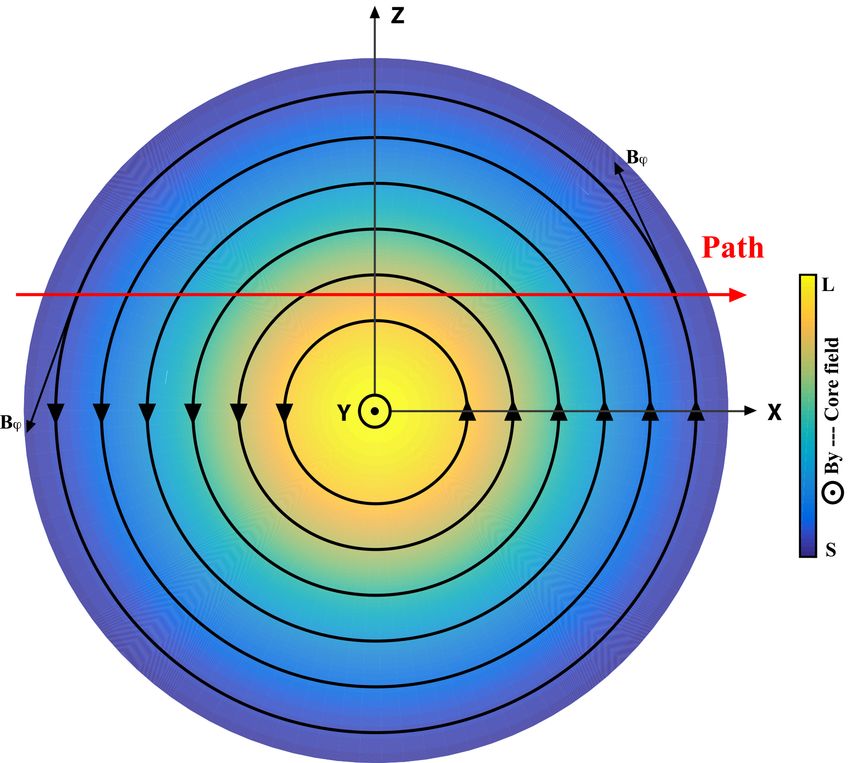
Finally, the candidates are fitted by a force-free model to de- Figure 1. Sketched diagram of the cylindrical flux rope. The flux
rope has a right-handed structure. The black circled lines are the
termine whether they belong to flux ropes or not.
magnetic field lines. The red arrow is the projection of spacecraft
For some flux ropes with short duration, the plasma data path. The rectangular coordinate is used in our analyses. Y is the
do not have enough high time resolution or, even worse, axis orientation of the flux rope, and the X–Z plane is the cross
are not available. Thus, the identification of flux ropes re- section perpendicular to the axis orientation. The core field is out
lies heavily on the magnetic field data. All aforementioned of plane, and the color represents the relative strength of core field
automatic methods are a bit complex, or require plasma data. (yellow: large, blue: small).
Therefore, to identify flux rope only using the magnetic field
data from a single spacecraft, we propose a new and simple
method based on the correlation coefficients between the sig-
nal and the ideal model of flux rope to identify flux ropes in
By = B(r) cos(α(r)),
space plasmas. The paper will be presented as follows: an in- Bϕ = B(r) sin(α(r)), (1)
troduction of the method in Sect. 2, the test of the method on
B(r) = B0 exp(−r 2 /b2 ),
artificial data from the model in Sect. 3, the applications of
the method on the Cluster and MMS data in Sect. 4, and the where α(r) = π/2(1 − exp(−r 2 /a 2 )); By is the core field
summary given in Sect. 5. component; B0 , a, and b are the constants; and r is the ra-
dial distance to the flux rope center.
Figure 1 shows a sketched diagram of the cylindrical flux
2 Approach rope from the E–R model. For convenience, the rectangular
coordinate is used in our analyses (shown in Fig. 1). Y is the
In this section, we simply introduce our method.
axis orientation of the flux rope, and the X–Z plane is the
Firstly, we derive the “target function to be correlated”
cross section perpendicular to the axis orientation. X can be
(TFC) from the ideal model of flux rope. Considering the
treated as Sun–Earth orientation, Y is the dawn–dusk orien-
variable and complicated observed flux ropes, we use the
tation, and Z is similar to the south–north orientation in the
ideal non-force-free model of flux rope proposed by Elphic
magnetotail. If one spacecraft crosses the flux rope follow-
and Russell (1983), named the Elphic and Russell (E–R)
ing the red path in Fig. 1, the Bz component will be charac-
model because most of flux ropes with nonnegligible perpen-
terized as bipolar signature, and the By component and total
dicular currents are not consistent with the force-free model
magnetic field Bt have strong peaks.
(e.g., Hidalgo et al., 2002; Zong et al., 2004; Zhang et al.,
Figure 2 shows the observations when one virtual space-
2010; Borg et al., 2012; Huang et al., 2012, 2016b). This
craft crosses the ideal flux rope (see spacecraft path in Fig. 1).
model is constructed with an intense core field inside of flux
Here we assume the scale of flux rope as one unit, and
rope, which is shown in Fig. 1. The equation of this model in
1 unit s−1 of moving speed of the spacecraft, thus set a =
the cylindrical coordinate (Y is defined as the axis orientation
0.735 units and b = 0.735 units, B0 = 10 nT, and use the Bz
of flux rope) can be modified as below:
as the bipolar variation component, By as the core field com-
ponent, Bt as the total magnetic field. The center of the flux
rope is located at 2.5 s. One can see the Bz bipolar signature,
Ann. Geophys., 36, 1275–1283, 2018 www.ann-geophys.net/36/1275/2018/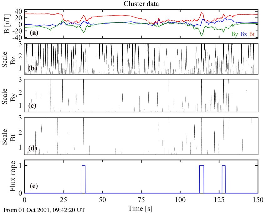
S. Huang et al.: A new method to identify flux ropes in space plasmas                                                                          1277

                                               E-R model                                         0.5
             2
                     (a)                                                                                   (a)
 B z [nT]

             0

                                                                                           Bz
                                                                                                  0
            -2

                                                                                                -0.5
             4 (b)
  B y [nT]

             2

             0                                                                                    1 (b)

                                                                                           By
             6                                                                                   0.5
                     (c)
             4
  B t [nT]

             2                                                                                    0
             0
                 0         0.5   1   1.5   2      2.5      3   3.5   4   4.5   5
                                                Time [s]
                                                                                                  1 (c)
Figure 2. The three variables Bz (a), By (b) and Bt (c) of the ideal

                                                                                            Bt
cylindrical flux rope described by the E–R model.                                                0.5

                                                                                                  0
                                                                                                       0         0.2   0.4     0.6   0.8   1
and the peaks of core field and total magnetic field inside the
                                                                                                                          Scale
flux rope.
   Considering the previous observations, in which the Bz                          Figure 3. The target-function-to-be-correlated (TFC) derived from
component during the crossing of the flux rope usually does                        E–R model. The amplitudes and scale are dimensionless.
not reach zero like that shown in Fig. 2a, we select one part
of the ideal flux rope as the TFC which is shown in Fig. 3.
The TFC is similar to the sinusoidal function when one per-                        nature in Bz , enhancements of core field By and magnetic
forms fast Fourier transform (FFT) analysis. We only used                          strength Bt should appear simultaneously with the same du-
two components (By and Bz ) and magnetic strength (Bt ) as                         ration when one spacecraft crosses the flux ropes.
the TFC since only Bz and By components and Bt have very                              Fourthly, we infer the location and the scale of the flux
obvious typical features usually from in situ measurements                         ropes based on the weighted average (it will be shown later),
(i.e., Bz has bipolar signature, By is strong core field, and Bt                   and the amplitude from minimum to maximum values of the
has peak inside flux ropes), and Bx component does not have                        bipolar variation.
common features from observation viewpoint (e.g., Slavin et
al., 2003; Huang et al., 2014a).
   Secondly, we calculate the Pearson correlation coefficients                     3   Model test
between the signal and the TFC at different times and differ-
ent scales (Hotelling, 1953). Before calculating the correla-                      One test is performed on the artificial data from E–R model
tion coefficients, the amplitude of the TFC will be estimated                      with the random noise. Figure 4 presents the test results. The
from the signal. For example, the maximum value of Bt dur-                         test artificial data are shown in Fig. 4a where the noise is
ing the time interval is used as the amplitude of Bt in the                        10 % of the amplitude of the flux rope. A series of the cal-
TFC. The sliding time window is used in the calculation of                         culations are carried on Bz , By and Bt to obtain the correla-
the correlation coefficients. The calculated results of corre-                     tion coefficients. One should point out that the absolute val-
lation coefficients are similar to the power spectral densities                    ues of the correlation coefficients of Bz and By are given
by FFT that display the power spectral density at different                        in Fig. 4b and c respectively, because the bipolar structure
times and different frequencies. The higher the values of the                      can be positive–negative or negative–positive variation and
correlation coefficients, the more suitable for the description                    the core field can be positive or negative. It can be seen that
of the model on the signal.                                                        the correlation coefficients are largest at the scale τ of 0.6–
   Thirdly, we compare the correlation coefficients of the                         1.5 units during the crossing of the flux rope (around time ∼
bipolar variation component Bz , core field component By                           3.5 s).
and total magnetic field Bt , and find out the high correla-                          We set the threshold as 0.9 to represent the results in Fig. 5
tions (larger than the given threshold) at the same time and                       where only the correlation coefficients with > 0.9 are dis-
the same scale. This is due to the fact that the bipolar sig-                      played with black shadows. All correlation coefficients of the

www.ann-geophys.net/36/1275/2018/                                                                                Ann. Geophys., 36, 1275–1283, 2018
1278                                                      S. Huang et al.: A new method to identify flux ropes in space plasmas

Figure 4. The test results on the E–R model. (a) Three variables Bz , By and Bt from E–R model with 10 % random noise; (b–d) the
correlation coefficients between the variables of Bz , By and Bt and the TFC shown in Fig. 3, respectively. The scale on the vertical axes of
(b–d) is τ , as mentioned in the text, which can also be seen as a unit.

three variables have peaks at the time ∼ 3.5 s with the scale            wave activities and electron-scale physics occur in the mag-
τ ∼ 1 units. We use the weighted-average technique (shown                netosheath ion-scale flux ropes. Figure 6 gives the observa-
below) to identify the flux rope and estimate its scale τ .              tions of ∼ 14 s from MMS2 on 25 October 2015 and the
     X               X                                                   test results of our method. The unit length of the TFC uses
τ=      coefi × τi /     coefi ,                            (2)          the same unit as the real observations, i.e., seconds (“s”).
                                                                         The amplitude (B0 ) of the TFC is determined by the max-
where coefi is the correlation coefficient at scale τi .                 imum value of Bt during the interval when calculating corre-
   Figure 5e shows the estimated results. The crossing of the            lation coefficients. Similar to the model test, we use the same
flux rope is marked with “1” and the duration is its scale, and          variables to present the components of the bipolar variation,
the center of the flux rope is at the center of the line. In this        core field and total magnetic field after transformed to MVA
test, the scale is estimated as 1.039 units, and the location is         (Huang et al., 2016b). The threshold of the correlation coeffi-
3.496 s. The amplitude is estimated to be 4.43 nT from min-              cients is also set as 0.9 in Fig. 6. We can see that the correla-
imum to maximum values of the bipolar variation. Afore-                  tion coefficients of the three variables (Fig. 6b–d) only have
mentioned sets, one can estimate the error of the scale as               high values at the same time around time = 5.5 s, implying
3.9 %, i.e., (1.039–1.0)/1.0 = 3.9 %. Therefore, our method              that one flux rope is identified by this method. Based on the
can successfully identify the flux rope and estimate its scale,          weighted-average method in Eq. (2), the timescale of the flux
location and amplitude.                                                  rope is 1.11 s, and its central location is at 5.38 s. The ampli-
                                                                         tude is estimated as 115 nT. All these results are consistent
4     Application                                                        with previous findings from multispacecraft data in Huang et
                                                                         al. (2016b).
In this section, we apply our new method to the spacecraft
measurements in the magnetosheath and the magnetotail.                   4.2   Flux rope in the magnetotail

4.1    Flux rope in the magnetosheath                                    Flux ropes are frequently observed in the magnetotail and
                                                                         play an important role during magnetic reconnection and
Flux ropes are successfully identified in the magnetosheath              magnetotail dynamics (e.g., Slavin et al., 2003; Zong et al.,
using the unprecedented high-resolution data from the MMS                2004; Chen et al., 2007; Huang et al., 2012, 2016a; Fu et al.,
(Burch et al., 2015) mission (Huang et al., 2016b). Their ob-            2015, 2016). Chen et al. (2008) have identified several flux
servations have demonstrated that highly dynamical strong-               ropes filled with energetic electrons during magnetic recon-

Ann. Geophys., 36, 1275–1283, 2018                                                               www.ann-geophys.net/36/1275/2018/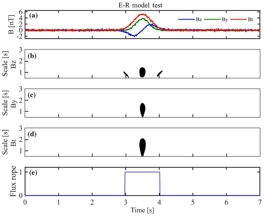
S. Huang et al.: A new method to identify flux ropes in space plasmas                                                                      1279

Figure 5. The test results on E–R model with a threshold of 0.9. (a) Three variables Bz , By and Bt from E–R model with 10 % random
noise; (b–d) the correlation coefficients (≥ 0.9) between the variables of Bz , By and Bt and the TFC, respectively; (e) the index when the
virtual spacecraft cross the flux rope (if the spacecraft cross the flux rope, the index is 1; if not, the index is 0). The duration of the index
presents the timescale of the flux rope. The scale on the vertical axes of (b–d) is the same as in Fig. 4.

Figure 6. Testing the method on MMS data in the magnetosheath. The same format as in Fig. 5. The scale on the vertical axes of (b–d) uses
seconds as the unit.

www.ann-geophys.net/36/1275/2018/                                                                   Ann. Geophys., 36, 1275–1283, 2018
1280                                                      S. Huang et al.: A new method to identify flux ropes in space plasmas

Figure 7. Testing the method on Cluster data in the magnetotail. The same format as in Fig. 6.

Table 1. The location, scale and amplitude of the flux ropes iden-      are available, then we can estimate the actual spatial scale
tified by the method. The amplitude is defined as the values of the     of the flux ropes. If multispacecraft data are available for the
bipolar variation from minimum to maximum.                              time interval of interest, one can derive the size, the orienta-
                                                                        tion and the motion of the flux rope using the multispacecraft
          No. of flux rope        1         2         3                 methods such as those of Sonnerup et al. (2004), Shi et al.
          Location (s)        37.91    113.79    127.93                 (2005, 2006) and Zhou et al. (2006a, b). However, the sepa-
          Scale (s)            1.99      2.84      2.05                 ration of the Cluster was much larger than the size of the flux
          Amplitude (nT)       9.96     20.49     12.59                 ropes on 1 October 2001, implying that one cannot use the
                                                                        multispacecraft method here.

nection on 1 October 2001 by using the Cluster data. Figure 7           5   Summary and discussion
shows the magnetic field in GSM coordinates from the Clus-
ter mission (Escoubet et al., 1997) in the magnetotail and              In summary, we developed a new method to identify flux
the application results of our method. There are several bipo-          ropes in the space plasmas. This method is based on the cor-
lar variations in Bz during this time interval (Fig. 7a). Fig-          relation coefficients between the signal and the TFC from the
ure 7b–d present the correlation coefficients (larger than 0.9          non-force-free E–R model. If the correlation coefficients of
of the threshold) of the three variables. Here we try to iden-          three variables (Bz , By and Bt ) of the signal have high values
tify small-scale flux ropes, so that we perform the method              of correlation coefficients at the same time and same scale,
only at short timescales. These are full of high correlation            one can deduce the existence of one flux rope and estimate its
coefficients (grey shadows in Fig. 7b–d). After compare with            location and its timescale (i.e., the duration). The tests on the
the correlation coefficients at the same time and same scale,           artificial data and the in situ realistic spacecraft data show
our method resolves three possible flux ropes in Fig. 7e. The           that our method can successfully search out the flux ropes
results are summarized in Table 1. The three structures are             and obtain their locations and timescales.
close to the ideal flux rope with bipolar signature in Bz , and            Bipolar variation in the Bz component and the enhance-
peaks in core field By and total magnetic field Bt . All three          ment in core field and magnetic field strength are the typical
flux ropes identified by our method have been reported in               signatures for most flux ropes. But it does not mean that all
Chen et al. (2007).                                                     observations from any crossing of the spacecraft would have
   We should point out that our method can only identify the            those signatures, which depends on the spacecraft trajectory
flux rope and derive its duration. If the plasma velocity data          (especially for bipolar components). However, one only can

Ann. Geophys., 36, 1275–1283, 2018                                                               www.ann-geophys.net/36/1275/2018/
S. Huang et al.: A new method to identify flux ropes in space plasmas 1281
select or identify the flux rope showing the typical signatures Data availability. MMS Data are publicly available from the MMS
and miss other flux rope that do not have the typical signa- Science Data Center at http://lasp.colorado.edu/mms/sdc/ (last ac-
tures. Some special field structures may induce similar sig- cess: September 2018). Cluster data are publicly available from the
natures along some special trajectories. But this opportunity Cluster Science Archive at http://www.cosmos.esa.int/web/csa (last
does not often occur in the magnetotail. Moreover, one can access: July 2018).
use the plasma measurements to rule out this possibility.
The aforementioned attempts are made to identify flux
Author contributions. SH and JH proposed the algorithm. PZ
ropes in the Earth’s magnetotail by eyes or half-automatically
coded the algorithm and tested and analyzed the algorithm output
based on the bipolar variation of Bz (e.g., Richardson et al.,
data. SH also helped with the algorithm development and analyzed
1987; Slavin et al., 2003; Kawano and Russell, 1996; Vogt et the data. RT and JB provided MMS data. SH wrote the paper, and
al., 2010; Jackman et al., 2014; Smith et al., 2016). The iden- all others commented on it.
tifications by eyes would miss a lots of flux ropes and take
too much time. Karimabadi et al. (2009) used a data mining
technique (MineTool) to search flux ropes using both mag- Competing interests. The authors declare that they have no conflict
netic field and plasma data. That method is too complex to of interest.
apply in the data analysis. Smith et al. (2017) proposed one
method to automatically detect force-free flux ropes based
on magnetic field data from a single spacecraft. In the present Acknowledgements. We thank the entire Cluster and MMS team
study, we used the TFC derived from non-force-free flux rope and instrument leads for data access and support. This work was
model to calculate the correlation coefficients with the signal, supported by the National Natural Science Foundation of China
and then compare the large correlation coefficients of differ- (41574168, 41674161, 41874191). Shiyong Huang acknowledges
ent variables to identify the flux rope. Our method is flexi- the support by Young Elite Scientists Sponsorship Program by
CAST (2017QNRC001).
ble, reliable and easy to apply with the in situ spacecraft data
compared with other methods. We will quantitatively model Edited by: Christopher Mouikis
the flux ropes identified by our method and derive more in- Reviewed by: two anonymous referees
formation on the flux ropes. For example, we can statistically
survey and investigate the locations, scales and global distri-
butions of flux ropes in the magnetosheath using MMS data.
References
We should point out that there are several limitations in
our method: Borg, A. L., Taylor, M. G. G. T., and Eastwood, J. P.: Ob-
servations of magnetic flux ropes during magnetic reconnec-
1. Our method can only detect the nearly ideal cylindrical tion in the Earth’s magnetotail, Ann. Geophys., 30, 761–773,
flux rope since we used non-force-free E–R model to https://doi.org/10.5194/angeo-30-761-2012, 2012.
describe the TFC, which limits the application of this Burch, J. L., Moore, T. E., Torbert, R. B., and Giles, B. L.: Magne-
method. The non-force-free model proposed by E–R is tospheric Multiscale overview and science objectives, Space Sci.
just one possible solution of all the flux rope that sat- Rev., 199, 5, https://doi.org/10.1007/s11214-015-0164-9, 2015.
isfies J × B 6 = 0. Actually, one can use other flux rope Chen, L.-J., Bhattacharjee, A., Puhl-Quinn, P. A., Yang, H.,
models to replace E–R model and extend our method Bessho, N., Imada, S., Mühlbachler, S., Daly, P. W., Lefebvre, B.,
to identify the flux ropes. Khotyaintsev, Y., Vaivads, A., Fazakerley, A., and Georgescu, E.:
Observation of energetic electrons within magnetic islands, Na-
2. If the flux ropes are not regular, there are large time de- ture Phys., 4, 19–23, https://doi.org/10.1038/nphys777, 2007.
viations among Bz , By and Bt that will lead to some flux Daughton, W., Scudder, J., and Karimabadi, H.: Fully ki-
ropes being missed when we apply the method. netic simulations of undriven magnetic reconnection with
open boundary conditions, Phys. Plasmas, 13, 072101,
3. The threshold value of correlation coefficients can affect https://doi.org/10.1063/1.2218817, 2006.
the results, such as when the threshold value is so small Deng, X. H., Matsumoto, H., Kojima, H., Mukai, T., An-
derson, R. R., Baumjohann, W., and Nakamura, R.: Geo-
that the method detects some possible structures that do
tail encounter with reconnection diffusion region in the
not belong to flux ropes, or so large that the method will
Earth’s magnetotail: Evidence of multiple X lines col-
miss some flux ropes. lisionless reconnection?, J. Geophys. Res., 109, A05206,
https://doi.org/10.1029/2003JA010031, 2004.
4. The correlation coefficients at small scales (especially
Drake, J. F., Swisdak, M., Che, H., and Shay, M. A.: Electron accel-
in By and Bt ) could be very large, which may affect eration from contracting magnetic islands during reconnection,
our results. The method may find some possible struc- Nature, 443, 553–556, 2006.
tures related to such fluctuations. We will improve this Elphic, R. C. and Russell, C. T.: Magnetic Flux Ropes in the Venus
method and apply it to detect the flux ropes in the tur- Ionosphere: Observations and Models, J. Geophys. Res., 88, 58–
bulent magnetosheath in the future. 72, https://doi.org/10.1029/JA088iA01p00058, 1983.
www.ann-geophys.net/36/1275/2018/ Ann. Geophys., 36, 1275–1283, 20181282 S. Huang et al.: A new method to identify flux ropes in space plasmas Escoubet, C. P., Schmidt, R., and Goldstein, M. L.: Cluster–Science netic reconnection, J. Geophys. Res.-Space Phys., 121, 205–213, and mission overview, Space Sci. Rev., 79, 11–32, 1997. https://doi.org/10.1002/2015JA021468, 2016a. Fu, H. S., Cao, J. B., Khotyaintsev, Yu. V., Sitnov, M. I., Runov, A., Huang, S. Y., Sahraoui, F., Retino, A., Le Contel, O., Yuan, Z. G., Fu, S. Y., Hamrin, M., André, M., Retinò, A., Ma, Y. D., Lu, H. Chasapis, A., Aunai, N., Breuillard, H., Deng, X. H., Zhou, M., Y., Wei, X. H., and Huang, S. Y.: Dipolarization fronts as a conse- Fu, H. S., Pang, Y., Wang, D. D., Torbert, R. B., Goodrich, K. A., quence of transient reconnection: In situ evidence, Geophys. Res. Ergun, R. E., Khotyaintsev, Y. V., Lindqvist, P.-A., Russell, C. Lett., 40, 6023–6027, https://doi.org/10.1002/2013GL058620, T., Strangeway, R. J., Magnes, W., Bromund, K., Leinweber, H., 2013. Plaschke, F., Anderson, B. J., Pollock, C. J., Giles, B. L., Moore, Fu, H. S., Vaivads, A., Khotyaintsev, Y. V., Olshevsky, V., An- T. E., and Burch, J. L.: MMS observations of ion-scale magnetic dré, M., Cao, J. B., Huang, S. Y., Retinò, A., and Lapenta, G.: island in the magnetosheath turbulent plasma, Geophys. Res. How to find magnetic nulls and reconstruct field topology with Lett., 43, 7850–7858, https://doi.org/10.1002/2016GL070033, MMS data?, J. Geophys. Res.-Space Phys., 120, 3758–3782, 2016b. https://doi.org/10.1002/2015JA021082, 2015. Hughes, W. J., Sibeck, D. G.: On the 3-dimensional structure of Fu, H. S., Cao, J. B., Vaivads, A., Khotyaintsev, Y. V., Andre, M., plasmoids, Geophys. Res. Lett., 14, 636–639, 2013. Dunlop, M., Liu, W. L., Lu, H. Y., Huang, S. Y., Ma, Y. D., and Jackman, C. M., Slavin, J. A., Kivelson, M. G., Southwood, D. J., Eriksson, E.: Identifying magnetic reconnection events using the Achilleos, N., Thomsen, M. F., DiBraccio, G. A., Eastwood, J. P., FOTE method, J. Geophys. Res.-Space Phys., 121, 1263–1272, Freeman, M. P., Dougherty, M. K., and Vogt, M. F.: Saturn’s dy- https://doi.org/10.1002/2015JA021701, 2016. namic magnetotail: A comprehensive magnetic field and plasma Fu, H. S., Vaivads, A., Khotyaintsev, Y. V., André, M., Cao, J. B., survey of plasmoids and traveling compression regions and their Olshevsky, V., Eastwood, J. P., and Retinò, A.: Intermittent en- role in global magnetospheric dynamics, J. Geophys. Res.-Space ergy dissipation by turbulent reconnection, Geophys. Res. Lett., Phys., 119, 5465–5494, https://doi.org/10.1002/2013JA019388, 44, 37–43, https://doi.org/10.1002/2016GL071787, 2017. 2014. Hidalgo, M. A., Cid, C., Vinas, A. F., and Sequeiros, J.: Karimabadi, H., Sipes, T. B., Wang, Y., Lavraud, B., and A non-force-free approach to the topology of magnetic Roberts, A.: A new multivariate time series data anal- clouds in the solar wind, J. Geophys. Res., 106, 1002, ysis technique: Automated detection of flux transfer https://doi.org/10.1029/2001JA900100, 2002. events using Cluster data, J. Geophys. Res., 114, A06216, Hotelling, H.: New Light on the Correlation Coefficient and its https://doi.org/10.1029/2009JA014202, 2009. Transforms, J. Roy. Stat. Soc. B, 15, 193–232, 1953. Kawano, H. and Russell, C. T.: Survey of flux transfer events ob- Hu, Q. and Sonnerup, B. U. O.: Reconstruction of magnetic flux served with the ISEE 1 spacecraft: Rotational polarity and the ropes in the solar wind, Geophys. Res. Lett., 28, 467–470, 2001. source region, J. Geophys. Res., 101, 27299–27308, 1996. Hu, Q. and Sonnerup, B. U. O.: Reconstruction of magnetic clouds Lee, L. C., Fu, Z. F., and Akasofu, S.-I.: A simulation study of in the solar wind: Orientations and configurations, J. Geophys. forced reconnection processes and magnetospheric storms and Res., 107, 1142, https://doi.org/10.1029/2001JA000293, 2002. substorms, J. Geophys. Res., 90, 10896–10910, 1985. Huang, S. Y., Vaivads, A., Khotyaintsev, Y. V., Zhou, M., Lepping, R. P., Jones, J. A., and Burlaga, L. F.: Magnetic field struc- Fu, H. S., Retinò, A., Deng, X. H., André, M., Cully, ture of interplanetary magnetic clouds at 1 AU, J. Geophys. Res., C. M., He, J. S., Sahraoui, F., Yuan, Z. G., and Pang, 95, 11957–11965, 1990. Y.: Electron acceleration in the reconnection diffusion re- Nakamura, M. and Scholer, M.: Structure of the magne- gion: Cluster observations, Geophys. Res. Lett., 39, L11103, topause reconnection layer and of flux transfer events: https://doi.org/10.1029/2012GL051946, 2012. Ion kinetic effects, J. Geophys. Res., 105, 23179–23191, Huang, S. Y., Pang, Y., Yuan, Z., Deng, X., He, J., Zhou, M., Fu, H., https://doi.org/10.1029/2000JA900101, 2000. Fu, S., Li, H., Wang, D., and Li, H.: Observation of directional Richardson, I. G., Cowley, S. W. H., Hones, E. W., and change of core field inside flux ropes within one reconnection Bame, S. J.: Plasmoid-associated energetic ion bursts in the diffusion region in the Earth’s magnetotail, Chin. Sci. Bull., 59, deep geomagnetic tail: Properties of plasmoids and the post- 4797–4803, https://doi.org/10.1007/s11434-014-0583-0, 2014a. plasmoid plasma sheet, J. Geophys. Res., 2, 9997–10013, Huang, S. Y., Zhou, M., Yuan, Z. G., Deng, X. H., Sahraoui, F., https://doi.org/10.1029/JA092iA09p09997, 1987. Pang, Y., and Fu, S.: Kinetic simulations of electric field structure Rong, Z. J., Wan, W. X., Shen, C., Zhang, T. L., Lui, A. T. Y., Wang, within magnetic island during magnetic reconnection and their Y., Dunlop, M. W., Zhang, Y. C., and Zong, Q.-G.: Method applications to the satellite observations, J. Geophys. Res.-Space for inferring the axis orientation of cylindrical magnetic flux Phys., 119, 7402–7412, https://doi.org/10.1002/2014JA020054, rope based on single-point measurement, J. Geophys. Res.-Space 2014b. Phys., 118, 271–283, https://doi.org/10.1029/2012JA018079, Huang, S. Y., Zhou, M., Yuan, Z. G., Fu, H. S., He, J. S., Sahraoui, 2013. F., Aunai, N., Deng, X. H., Fu, S., Pang, Y., and Wang, D. Slavin, J. A., Lepping, R. P., Gjerloev, J., Fairfield, D. H., Hesse, M., D.: Kinetic simulations of secondary reconnection in the re- Owen, C. J., Moldwin, M. B., Nagai, T., Ieda, A., and Mukai, T.: connection jet, J. Geophys. Res.-Space Phys., 120, 6188–6198, Geotail observations of magnetic flux ropes in the plasma sheet, https://doi.org/10.1002/2014JA020969, 2015. J. Geophys. Res., 108, 1015–1032, 2003. Huang, S. Y., Retino, A., Phan, T. D., Daughton, W., Vaivads, A., Shi, Q. Q., Shen, C., Pu, Z. Y., Dunlop, M. W., Zong, Q.-G., Zhang, Karimabadi, H., Zhou, M., Sahraoui, F., Li, G. L., Yuan, Z. G., H., Xiao, C. J., Liu, Z. X., and Balogh, A.: Dimensional analysis Deng, X. H., Fu, H. S., Fu, S., Pang, Y., and Wang, D. D.: In of observed structures using multipoint magnetic field measure- situ observations of flux rope at the separatrix region of mag- Ann. Geophys., 36, 1275–1283, 2018 www.ann-geophys.net/36/1275/2018/
S. Huang et al.: A new method to identify flux ropes in space plasmas                                                                  1283

  ments: Application to Cluster, Geophys. Res. Lett., 32, L12105,       Wang, R., Lu, Q., Nakamura, R., Huang, C., Du, A., Guo, F., Teh,
  https://doi.org/10.1029/2005GL022454, 2005.                             W., Wu, M., Lu, S., and Wang, S.: Coalescence of magnetic flux
Shi, Q. Q., Shen, C., Dunlop, M. W., Pu, Z. Y., Zong, Q.-G.,              ropes in the ion diffusion region of magnetic reconnection, Na-
  Liu, Z.-X., Lucek, E. A., and Balogh, A.: Motion of observed            ture Phys., 12, 263–267, https://doi.org/10.1038/nphys3578,
  structures calculated from multi-point magnetic field measure-          2016.
  ments: Application to Cluster, Geophys. Res. Lett., 33, L08109,       Zhang, H., Kivelson, M. G., Khurana, K. K., McFadden, J.,
  https://doi.org/10.1029/2005GL025073, 2006.                             Walker, R. J., Angelopoulos, V., Weygand, J. M., Phan,
Smith, A. W., Jackman, C. M., and Thomsen, M. F.: Magnetic re-            T., Larson, D., Glassmeier, K. H., and Auster, H. U.: Ev-
  connection in Saturn’s magnetotail: A comprehensive magnetic            idence that crater flux transfer events are initial stages of
  field survey, J. Geophys. Res.-Space Phys., 121, 2984–3005,             typical flux transfer events, J. Geophys. Res., 115, A08229,
  https://doi.org/10.1002/2015JA022005, 2016.                             https://doi.org/10.1029/2009JA015013, 2010.
Smith, A. W., Slavin, J. A., Jackman, C. M., Fear, R. C., Poh, G.-K.,   Zhou, X.-Z., Zong, Q.-G., Pu, Z. Y., Fritz, T. A., Dunlop, M.
  DiBraccio, G. A., Jasinski, J. M., and Trenchi, L. (2017), Auto-        W., Shi, Q. Q., Wang, J., and Wei, Y.: Multiple Triangu-
  mated force free flux rope identification,J. Geophys. Res.-Space        lation Analysis: another approach to determine the orienta-
  Phys., 122, 780–791, https://doi.org/10.1002/2016JA022994,              tion of magnetic flux ropes, Ann. Geophys., 24, 1759–1765,
  2017.                                                                   https://doi.org/10.5194/angeo-24-1759-2006, 2006a.
Sonnerup, B. U. O., Hasegawa, H., and Paschmann, G.: Anatomy            Zhou, X.-Z., Zong, Q.-G., Wang, J., Pu, Z. Y., Zhang, X. G., Shi,
  of a flux transfer event seen by Cluster, Geophys. Res. Lett., 31,      Q. Q., and Cao, J. B.: Multiple triangulation analysis: appli-
  L11803, https://doi.org/10.1029/2004GL020134, 2004.                     cation to determine the velocity of 2-D structures, Ann. Geo-
Vogt, M. F., Kivelson, M. G., Khurana, K. K., Joy, S. P., and Walker,     phys., 24, 3173–3177, https://doi.org/10.5194/angeo-24-3173-
  R. J.: Reconnection and flows in the Jovian magnetotail as in-          2006, 2006b.
  ferred from magnetometer observations, J. Geophys. Res., 115,         Zong, Q.-G., Fritz, T. A., Pu, Z. Y., Fu, S. Y., Baker, D. N., Zhang,
  A06219, https://doi.org/10.1029/2009JA015098, 2010.                     H., Lui, A. T., Vogiatzis, I., Glassmeier, K.-H., Korth, A., Daly,
Wang, R., Lu, Q., Du, A., and Wang, S.: In Situ Observations of a         P. W., Balogh, A., and Reme, H.: Cluster observations of earth-
  Secondary Magnetic Island in an Ion Diffusion Region and Asso-          ward flowing magnetic island in the tail, Geophys. Res. Lett., 31,
  ciated Energetic Electrons, Phys. Rev. Lett., 104, 175003, 2010.        L18803, https://doi.org/10.1029/2004GL020692, 2004.

www.ann-geophys.net/36/1275/2018/                                                                Ann. Geophys., 36, 1275–1283, 2018
You can also read