Tsunami generated magnetic fields have primary and secondary arrivals like seismic waves - Nature
←
→
Page content transcription
If your browser does not render page correctly, please read the page content below
www.nature.com/scientificreports
OPEN Tsunami‑generated magnetic
fields have primary and secondary
arrivals like seismic waves
Takuto Minami1, Neesha R. Schnepf2,3 & Hiroaki Toh4*
A seafloor geomagnetic observatory in the northwest Pacific has provided very long vector
geomagnetic time-series. It was found that the time-series include significant magnetic signals
generated by a few giant tsunami events including the 2011 Tohoku Tsunami. Here we report that
the tsunami-generated magnetic fields consist of the weak but first arriving field, and the strong but
second arriving field—similar to the P- and S-waves in seismology. The latter field is a result of coupling
between horizontal particle motions of the conductive seawater and the vertical component of the
background geomagnetic main field, which have been studied well so far. On the other hand, the
former field stems from coupling between vertical particle motions and the horizontal component
of the geomagnetic main field parallel to tsunami propagation direction. The former field has been
paid less attention because horizontal particle motions are dominant in the Earth’s oceans. It,
however, was shown that not only the latter but also the former field is significant especially around
the magnetic equator where the vertical component of the background magnetic field vanishes. This
implies that global tsunami early warning using tsunami-generated magnetic fields is possible even in
the absence of the background vertical geomagnetic component.
A devastating tsunamigenic earthquake of Mw9.1 occurred on the landward slope of the Japan Trench on March
11, 2011 (Table 1), which resulted in enormous damage to Japanese society not only by its very strong seismic
motions but also its gigantic tsunami. Seismic and tsunami data of this large earthquake have been studied
intensively to yield its focal and tsunami source mechanisms1. Its tsunami was also detecteded2,3 by the seafloor
geomagnetic observatory4,5 operating on the northwest Pacific Basin even at a large epicentral distance of more
than 1500 km (Fig. 1). It was found that the seafloor observatory detected significant magnetic signals generated
by a few giant tsunami events6,7 including that of the 2011 Tohoku Earthquake2. Those detections were enabled
through the so-called motional induction e ffect8, which was first studied by F araday9. Since then, study of this
effect had been mainly focused on non-transient oceanic motions such as tides10–13 and the western boundary
currents14–16. However, the time scale of tsunamis is much shorter than that of the long-period currents and
thus temporal variations of the tsunami-generated magnetic fields should be considered explicitly in solving the
induction equation for magnetic fields in either the f requency6 or time 2,3 domain.
Results
Figure 1b clearly shows that the 2011 off the Pacific coast of Tohoku Earthquake emitted tsunamis that can be
identified by magnetic variations as large as 3nT even at a very large epicentral distance (1536 km; Table 1). The
time variations are evident mainly in the eastward and downward magnetic components, because the tsunamis
propagated towards east from the epicentre to the seafloor site (NWP; Fig. 1a and Fig. S1a). At NWP, the mag-
netometer sensed the eastward and downward components since the tsunami-generated electric currents were
concentrated along the tsunami wave front that oriented in the north–south direction around NWP (Fig. S1b).
Even though geomagnetic variations on the seafloor are less subject to external fields, the observed raw time series
(the red curves in Fig. 1b) were corrected by a transfer function method4 between NWP and a remote reference
site (MMB) using very long time-series of non-tsunami periods to yield cleaned time-series (the green curves).
It has been pointed out that the wavelet analysis is a powerful tool to detect geomagnetic d isturbances17,18. The
cleaned time-series, therefore, were further analysed by a cross-wavelet analysis method (Fig. 1c), which suc-
cessfully identified the co-tsunami magnetic variation even in the presence of a moderate external disturbance
1
Graduate School of Science, Kobe University, Nada‑ku, Kobe 6578501, Japan. 2Cooperative Institute for Research
in Environmental Sciences (CIRES), University of Colorado, Boulder, CO 80309‑0216, USA. 3Department of
Geological Sciences, University of Colorado, Boulder, CO 80309‑0216, USA. 4Graduate School of Science, Kyoto
University, Sakyo‑ku, Kyoto 6068502, Japan. *email: tou.hiroaki.7u@kyoto‑u.ac.jp
Scientific Reports | (2021) 11:2287 | https://doi.org/10.1038/s41598-021-81820-5 1
Vol.:(0123456789)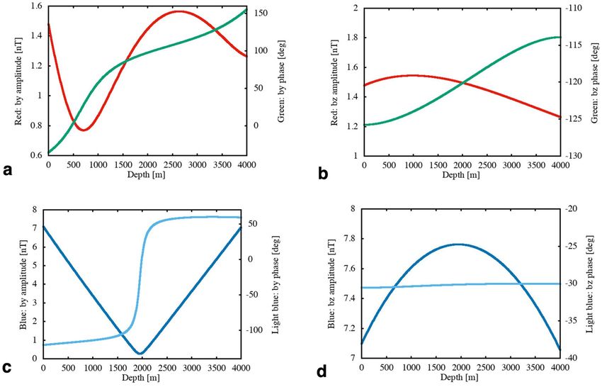
www.nature.com/scientificreports/
Origin time Moment magnitude (Mw)
Latitude (oN) Longitude (oE) Depth (km) Epicentral distances (km) Site names
38.297 142.373 29.0 March 11, 2011 05:46:24 UTC 9.1*
41.102 159.963 5.58 1535.8 NWP
43.910 144.189 − 0.042 643.1 MMB
Table 1. Earthquake and site descriptions. *Details of the tsunamigenic earthquake can be obtained from
United States Geological Survey (USGS) at https://earthquake.usgs.gov/earthquakes/eventpage/official2011031
1054624120_30/executive.
manifested in Kp indices19 on March 11, 2011. It is evident in Fig. 1d that there exist no significant signals in the
cross-wavelet result before the tsunami arrival.
The presence of a significant tsunami-generated magnetic signal in the cleaned time-series is indisputable
as shown in Fig. 1c. However, the phase relation between the tsunami wave height and the tsunami-generated
magnetic field is not very clear in this plot. We, therefore, used an analytical solution of the tsunami-generated
electromagnetic (EM) fields in the frequency domain to clarify whether the magnetic field has an identifiable
phase lag or lead with respect to tsunami wave height. Detailed derivation of the analytical solution utilized here
is described in the ‘Methods Section’.
Analytical solutions of tsunami-generated EM fields in the frequency domain have been obtained by several
works20–22. However, the majority of the preceding works neglected the source electromotive force arising from
coupling of the horizontal geomagnetic component (Fy) with the vertical flow velocity (vz) of the conductive
seawater. Instead, they focused on the coupling of the vertical geomagnetic component (Fz) with the horizontal
flow velocity (vy), which may have been a natural choice, to first-order approximation, because vy is several times
larger than vz in the case of tsunamis. Our point here, however, is that the vzFy coupling cannot be neglected in
the sense that not only does it create a large phase lead of the tsunami-generated EM fields with respect to the
kinetic phase of tsunamis but it also does not vanish to zero amplitude—even in the equatorial regions where
Fz tends to become very small.
We plotted the contribution of the vzFy coupling in the upper two panels of Fig. 2, while the vyFz coupling
is shown in the lower panels. The magnitudes of the ambient geomagnetic components were set identical for
both couplings for easier comparison. The left two panels of Fig. 2 show the by component, while the right
panels show bz. Comparing the amplitudes of the tsunami-generated magnetic components, the vzFy coupling
gives ~ 1.5nT at most, whereas the vyFz coupling can create 7 ~ 8nT—4–5 times more than the vzFy coupling. All of
the tsunami-generated magnetic components are subject to significant changes in amplitude through the ocean
layer. Especially for the vzFy coupling, the depth dependence of the tsunami-generated magnetic components
in a uniformly conducting ocean is governed by a combination of the different reflection of the EM fields in the
ocean at the seafloor and at the sea surface, and the almost linear decrease of vz with depth from a finite value at
the sea surface to nil at the seafloor. It is noteworthy that the amplitude ratio, bz (or by) by the vyFz coupling to
those by the vzFy coupling, is nearly equal to that of the flow velocity (vy/vz ~ 5).
The phase lag of the tsunami-generated magnetic components with respect to the tsunami wave height also
has depth dependence. According to Fig. 2a–d, every component has larger lags at depth compared with those
near the sea surface. Note that the phase difference is given as ‘phase lag’ in Fig. 2, so the negative values actu-
ally correspond to ‘phase lead’. The bz component arising from the vyFz coupling (Fig. 2d) possesses the largest
amplitude (~ 7.8 nT in the middle of the ocean layer). However, its phase lead is only 30 degrees for the 3 mHz
frequency used in the calculation. This means that the largest tsunami-generated magnetic signal arrives just
before the actual tsunami arrival. The phase lead is equivalent to only a one-twelfth of the tsunami period, which
is equal to slightly less than 28 s. The same argument is applicable to the by component arising from the vzFy
coupling (Fig. 2a), which possesses large phase lags in most of the ocean layer but turns to ‘lead’ of less than 40
degrees near the sea surface.
The largest phase lead is realized by the bz component arising from the vzFy coupling (Fig. 2b). It reaches a
lead as large as 125 degrees—equivalent to more than one-third of the tsunami period. Namely, we can observe
a small but significant (more than 1 nT) tsunami-generated magnetic signal 116 s (~ 2 min) prior to the actual
tsunami arrival in this case. Another significant phase lead is achieved by the by component arising from the vyFz
coupling (Fig. 2c), which possesses a large amplitude (~ 7nT) but the large phase lead (~ 120 degrees) can only
be observed on the sea surface and not on the seafloor. The reason why the vzFy coupling leads the vyFz coupling
by approximately 90 degrees in phase lies in the fact that vz has maximum amplitude at the wave’s nodes (see
Fig. S2) while vy does at the peaks.
Actual phase lead of the magnetic variation at the time of tsunami first arrival should be investigated more
carefully since the phase relationship mentioned above is based on the continuous sinusoidal tsunami and the
analytical solution is given in frequency domain. We, therefore, modelled magnetic variation due to a synthetic
(but realistic) tsunami first arrival, which consists of a large main tsunami peak of 1 m and a preceding small
negative peak of 0.1 m due to elasticity of the E arth23. See “Method” section for details of the solution in time
domain. Figure 3 shows the result of the modelling, where bz due to the vz Fy and vy Fz couplings are compared
with the adopted tsunami waveform. The characteristic frequency of the tsunami first arrival is ~ 3 mHz and
the tsunami height of the main peak is ~ 1 m. Results from the modelling, therefore, are comparable to those
shown in Fig. 2.
Scientific Reports | (2021) 11:2287 | https://doi.org/10.1038/s41598-021-81820-5 2
Vol:.(1234567890)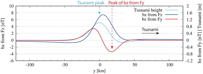
www.nature.com/scientificreports/
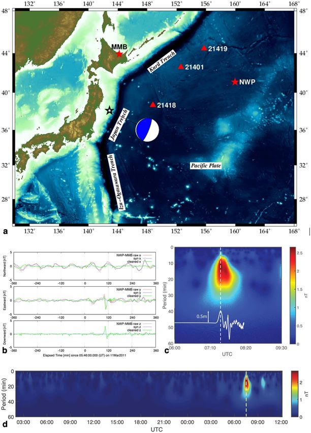
Figure 1. Site map, observed time-series and cross-wavelet analysis results. (a) The focal mechanism (the beach
ball*) of the 2011 off the Pacific coast of Tohoku Earthquake and its epicenter. Stars indicate the locations of our
seafloor EM station (NWP) and the reference geomagnetic observatory on land (MMB). Triangles show the
closest three DART** buoys. This figure was newly created by one of the authors (T.M.) using a combination
of public domain software and data, viz., Generic Mapping Tools (GMT)24 v.6.1.1 (https://www.generic-mappi
ng-tools.org/) and the global 1 min digital topography v.19.1 (https://topex.ucsd.edu/WWW_html/mar_topo.
html). (b) High-passed raw vector geomagnetic data (red), synthetic variations of external origin (blue), and the
difference (green = red–blue) at NWP. The synthetic variations were calculated using the transfer function that
casts the external geomagnetic field at MMB to that at NWP. The raw geomagnetic data were high pass filtered
with a cut-off period of 2 h. (c) The 3.5-h periodogram by our cross-wavelet analysis method17 for the difference
data of bz (the bottom green curve in b). This analysis used a maximum cut-off period of 30 min. The vertical
dashed line indicates the estimated time of arrival of the tsunami at NWP (07:30 UTC). The white line shows
a result of kinetic simulation for the 2011 Tohoku tsunami. (d) Same as (c) but for a longer duration (21 h) to
show the non-tsunami-related variations as well. *https://earthquake.usgs.gov/earthquakes/eventpage/official20
110311054624120_30/moment-tensor **https://www.ndbc.noaa.gov/dart.shtml.
Scientific Reports | (2021) 11:2287 | https://doi.org/10.1038/s41598-021-81820-5 3
Vol.:(0123456789)www.nature.com/scientificreports/
Figure 2. Analytical solutions arising from either Fy or Fz of the ambient field. a, Amplitude (red) and phase
(green) curves of the horizontal magnetic component (by) generated by the vzFy coupling within a flat ocean of
4000 m depth over a uniform half space of 0.01S/m conductivity. Phases are given as ‘lag’ w.r.t. the maximum
tsunami wave height. (b) Same as (a) but for the downward magnetic component (bz). (c) Amplitude (blue)
and phase (light blue) curves of the horizontal magnetic component (by) generated by the vyFz coupling. This
component retains opposite signs and the maxima of amplitudes on both sides of the ocean. The presence of
conductive substrata results in a slight deviation from the perfect symmetry with respect to the half ocean depth
(2000 m). (d) Same as (c) but for the downward magnetic component (bz). Note that the sign of bz by the vz Fy
coupling is flipped to make it correspond to the peak of vz that has a π/2 phase lead w.r.t. tsunami wave height.
The wave height, A, is 1 m and the frequency is 3 mHz. We used 4S/m for the electrical conductivity of the
seawater and assumed the strength of the ambient geomagnetic field to be Fy = Fz = 35,000nT.
Figure 3. Predicted phase lead of bz by the vz F y coupling of the solitary wave. Predicted vertical components
of the magnetic variation at the seafloor, caused by coupling of vy Fz (bz from Fz ) and vz Fy (bz from Fy ). Refer to
the left ordinate for bz from Fz and right for both bz from Fy and the tsunami height. Fy = Fz = 35000nT are
adopted in the calculation. Ocean depth is set to 4000 m. See the “Methods” section for the derivation of the
tsunami wave form and how the magnetic variations are calculated. The negative peak of “bz from Fy ” clearly
precedes the peak of solitary tsunami and that of “bz from Fz”.
Scientific Reports | (2021) 11:2287 | https://doi.org/10.1038/s41598-021-81820-5 4
Vol:.(1234567890)www.nature.com/scientificreports/
Figure 3 illustrates that bz from vz F y has a definite advantage in its phase lead, though the amplitude and
the phase lead are smaller than expected by the analytical solution shown in Fig. 2b. As for bz from vy Fz , the
amplitude reaches 7nT and the phase lead amounts to 6 km distance with respect to the tsunami main peak,
namely about 30 s ahead in time. As for bz from vz Fy , the amplitude is ~ 0.6nT and the negative peak precedes
the tsunami main peak by 19 km, namely 96 s (1.6 min) in time. The amplitude is about a half and the phase
lead is almost comparable to the results from Fig. 2b. Although the phase lead of bz from vz Fy is slightly smaller
than that expected by the frequency domain solution, the negative peak is still earlier than the main peak of bz
from vy Fz more than one and half minutes.
Discussion
It seems promising to observe the by component arising from the vyFz coupling on the sea surface for the purpose
of tsunami early warning. Oceanic islands in the mid- to high-latitudes can be regarded as the ideal locations to
observe the large phase lead, provided that the site effect in the vicinity of those islands can be corrected prop-
erly. However, the by component arising from the vyFz coupling is inevitably associated with the following two
drawbacks: (1) No signal can be detected in the equatorial regions since it consists solely of the Fz contribution.
(2) External geomagnetic disturbances are much more abundant in the horizontal geomagnetic components
than in the vertical component, which can mask the tsunami-generated signals easily.
On the contrary, the bz component arising from the vzFy coupling is strongest (see Fig. S3) on the magnetic
equator in terms of the source electromotive force, and it has the largest phase lead among the four components
(see Figs. 2a–d). Furthermore, external geomagnetic disturbances contain less of the vertical component, espe-
cially in mid-latitudes. Another source of magnetic noise in the vertical component is the electrical structure-
dependent horizontal shear of the electric currents flowing both in the ocean and beneath the seafloor that are
induced by external disturbances. However, as depicted in Fig. 1b, the effect of EM induction within both the
ocean and the solid Earth can be reduced considerably using magnetic data without tsunami events.
Our time domain solution shown in Fig. 3 has revealed that the phase lead of bz by vz Fy is slightly smaller than
that in frequency domain but still there. The expected phase lead of ~ 2 min in the analytical solution is reduced
to 1.6 min for the tsunami first arrival. We speculate that this comes from the difference between solitary waves
and continuous sinusoidal waves; the lack of a large negative peak (~ 1 m) preceding the tsunami main peak
results in the phase delay and decreases the amplitude of vz and thereby those of bz by vz Fy . Our time-domain
modelling also demonstrated that the vz Fy coupling generates bz with a detectable amplitude (~ 0.6 nT on the
seafloor and ~ 0.8 nT on the sea surface) and with a larger phase lead than that of bz by vy Fz . In the vicinity of
the geomagnetic equator, this effect plays a dominant role in the tsunami-generated magnetic variation because
Fz diminishes virtually there.
Considering the protection against external disturbances argued above, the bz components are better choices
than the by components. If we select to observe the tsunami-generated bz component either on the sea surface
or on the seafloor, we first detect a small magnetic signal stemming from the vzFy coupling earlier than the
actual tsunami arrival. The small but significant signal will be followed by a much larger signal arising from the
vyFz coupling that will be observed just before the tsunami arrival. Those primary and secondary arrivals of the
tsunami-generated bz component are quite similar to the well-known P- and S-arrivals of seismic waves and can
be observed both on the sea surface and on the seafloor.
Conclusions
Generation of EM fields by conductive geofluid moving through the ambient geomagnetic field has been studied,
since the EM induction phenomenon itself was first d iscovered9. Many types of ocean flows, such as tides or the
western boundary currents, in addition to t sunamis3 have been proved to have motionally induced EM fields.
However, most of previous works were focused on the vertical component of the ambient geomagnetic field,
neglecting the horizontal geomagnetic component. Here we show that the coupling of the horizontal geomag-
netic component with the vertical particle motion of the conductive seawater can generate observable vertical
magnetic signals with significant phase lead to the tsunami wave height. Furthermore, we find that the vertical
magnetic signal is followed by another vertical magnetic signal of larger amplitude just before the tsunami arrival.
This pair of vertical magnetic signals generated by tsunamis is analogous to the pair of seismic P- and S-waves
generated by earthquakes. Because those vertical magnetic signals have better protection against geomagnetic
disturbances of external origin and the fast-arriving signal is ubiquitous over the globe (i.e., it never vanishes
even on the dip equator), the pair of magnetic signals can be applied to global tsunami early warning systems
for disaster mitigation. Even though a few minutes seem too short, they are long enough to give alerts for people
at the coast to evacuate.
Methods
Analytical solution of tsunami‑generated EM fields for linear dispersive waves. Analytical solu-
tions of tsunami-generated EM fields in the frequency domain can be derived if analytical forms of the tsunami’s
velocity fields are known. Here we adopt two-dimensional linear dispersive waves with wave fronts parallel to
the x-direction and propagating toward the y-direction over a flat ocean of a constant depth of h with a down-
ward positive z-axis. The origin of z-axis is set at the averaged sea surface. We further assume that the seawater
is incompressible and the flow is irrotational, which means that there exists a velocity potential, Ф, for this flow.
It follows that Ф is a harmonic function that obeys the following Laplace equation:
= 0. (1)
It can be readily shown that Ф has an analytical form of
Scientific Reports | (2021) 11:2287 | https://doi.org/10.1038/s41598-021-81820-5 5
Vol.:(0123456789)www.nature.com/scientificreports/
ω cosh(k(z − h)) i(ky−ωt )
� = −iA e , (2)
k sinh(kh)
provided that the time- and y-dependence of Ф is ei(ky−ωt ), and that the energy conservation and linear bound-
ary conditions are imposed on both the sea surface and seafloor. The wave number and angular frequency of the
linear dispersive wave in concern are denoted by k and ω, respectively. A is the height of the linear dispersive
wave. The dispersion relation of the linear dispersive wave is given by.
ω2 g
2
= tanh(kh), (3)
k k
where g is the gravitational acceleration on the Earth’s surface.
The governing equation of the tsunami-generated magnetic field, b, in a medium of constant electrical con-
ductivity, σ, can be written as
2
(4)
∇ − iωσ µ0 b = −σ µ0 ∇ × (v × F),
where µ0 is the magnetic permeability of the medium, while v and F are the particle velocity of the linear disper-
sive wave and the ambient magnetic field (|b|<www.nature.com/scientificreports/
αl e(αl+1 −αl )zl + αl+1 e(αl+1 −αl )zl αl e−(αl+1 +αl )zl − αl+1 e−(αl+1 +αl )zl
Cl 1 Cl+1
= (11)
Dl 2αl αl e(αl+1 +αl )zl − αl+1 e(αl+1 +αl )zl αl e−(αl+1 −αl )zl + αl+1 e−(αl+1 −αl )zl Dl+1
The analytical solutions in eqs. (6) through (8) are a complete set of the two-dimensional wave field in the
sense that the source electromotive force and the induced electric field lie in the x-direction alone to generate
the magnetic field in the yz-plane. Each set of ζi and ψi (i = x, y or z) can be interpreted as transfer functions
that represent the contribution of the ambient geomagnetic field (Fz or Fy) to the tsunami-generated magnetic
field, b. The solutions are also ‘complete’ because they explicitly contain the contribution of Fy (i.e., ψi), which
has been neglected in most of the previous works. The contribution of the horizontal geomagnetic component
in the background is especially important in the equatorial regions where the vertical geomagnetic component
vanishes. We used eqs. (7) and (8) to make the plots in Fig. 2.
Time domain modelling of tsunami‑generated EM variations using solitary waves. The phase
lead in the time domain of the magnetic variation can be investigated by semi-analytical modelling using solitary
wave forms. Sea surface elevation of a solitary wave, η, can be expressed as
2 y − ct
′
η(y, t) = A sech (12)
L
where A′ is the peak height of the wave, c is the phase velocity, L is the horizontal scale length of the solitary wave.
Defining the following Fourier transform and its inverse,
−
∞ ∞
(13)
f (k, ω) = dt dyf y, t exp −iky + iωt
−∞ −∞
∞
∞ −
f y, t = (2π)−2 (14)
dω dk f (k, ω)exp iky − iωt ,
−∞ −∞
the solitary wave in the frequency-wave number domain is given by:
− 2π 2 AL2 k
η (k, ω) = δ(ω − kc). (15)
sinh(πLk/2)
The magnetic variation generated by the solitary wave can be evaluated by substitution of Eq. (15) into A
in Eq. (7) or (8) and their numerical integrations in Eq. (14). Figure 3 shows the results for bz by Fz and Fy and
their phase relation in the time domain. In Fig. 3, superposition of two solitary waves is used for generation of
the realistic tsunami first arrival, which includes a small initial negative polarity in the tsunami first a rrival24. As
a result, the adopted tsunami wave form is expressed by
2
2 y − ct − yi
′
η y, t = Ai sech , (16)
Li
i=1
where (A′ 1 , A′ 2 ) = (1.1, −0.3)m, y1 , y2 = (1, 25)km, and L1 = L2 = 18km. The resulting horizontal distance
from the initial negative peak to the main positive one is 34 km. The characteristic frequency of the tsunami is
therefore ~ 3 mHz, which is derived by Eq. (3) with the wavelength of 68 km.
Received: 8 June 2020; Accepted: 11 January 2021
References
1. Satake, K. et al. Time and space distribution of coseismic slip of the 2011 Tohoku earthquake as inferred from tsunami waveform
data. Bull. Seismol. Soc. Am. 103(2B), 1473–1492. https://doi.org/10.1785/0120120122 (2013).
2. Minami, T. & Toh, H. Two-dimensional simulations of the tsunami dynamo effect using the finite element method. Geophys. Res.
Lett. 40, 4560–4564 (2013).
3. Minami, T. et al. Three-dimensional time domain simulation of tsunami-generated electromagnetic fields: application to the 2011
Tohoku earthquake tsunami. J. Geophys. Res. 122, 9559–9579. https://doi.org/10.1002/2017JB014839 (2017).
4. Toh, H. et al. Geomagnetic observatory operates at the seafloor in the northwest Pacific Ocean. Eos Trans. AGU85, 467–473 (2004).
5. Toh, H., Hamano, Y. & Ichiki, M. Long-term seafloor geomagnetic station in the northwest Pacific: a possible candidate for a
seafloor geomagnetic observatory. Earth Planets Space 58, 697–705 (2006).
6. Kawashima, I. & Toh, H. Tsunami-generated magnetic fields may constrain focal mechanisms of earthquakes. Sci. Rep. 6, 28603.
https://doi.org/10.1038/srep28603 (2016).
7. Toh, H. et al. Tsunami signals from the 2006 and 2007 Kuril earthquakes detected at a seafloor geomagnetic observatory. J. Geophys.
Res. 116, B02104. https://doi.org/10.1029/2010JB007873 (2011).
8. Sanford, T. B. Motionally induced electric and magnetic fields in the sea. J. Geophys. Res. 76, 3476–3492 (1971).
9. Faraday, M. Experimental researches in electricity. Philos. Trans. R. Soc. Lond. 122, 174–177 (1832).
10. Malin, S. R. C. Separation of lunar daily geomagnetic variations into parts of ionospheric and oceanic origin. Geophys. J. R. Astr.
Soc. 21, 447–455 (1970).
11. Tyler, R. H., Maus, S. & Lühr, H. Satellite observations of magnetic fields due to ocean tidal flow. Science 299(5604), 239–241. https
://doi.org/10.1126/science.1078074 (2003).
Scientific Reports | (2021) 11:2287 | https://doi.org/10.1038/s41598-021-81820-5 7
Vol.:(0123456789)www.nature.com/scientificreports/
12. Schnepf, N. R. et al. Tidal signals in ocean-bottom magnetic measurements of the Northwestern Pacific: observation versus predic-
tion. Geophys. J. Int. 198, 1096–1110. https://doi.org/10.1093/gji/ggu190 (2014).
13. Schnepf, N. R. et al. A comparison of model-based ionospheric and ocean tidal magnetic signals with observatory data. Geophys.
Res. Lett. 45, 1–11. https://doi.org/10.1029/2018GL078487 (2018).
14. Larsen, J. C. & Sanford, T. B. Florida current volume transports from voltage measurements. Science 227, 302–304. https://doi.
org/10.1126/science.227.4684.302 (1985).
15. Manoj, C., Kuvshinov, A. & Maus, S. Ocean circulation generated magnetic signals. Earth Planets Space 58, 429–437 (2006).
16. Velímský, J., Šachl, L. & Martinec, Z. The global toroidal magnetic field generated in the Earth’s oceans. Earth Planet. Sci. Lett. 509,
47–54. https://doi.org/10.1016/j.epsl.2018.12.026 (2019).
17. Schnepf, N. R. et al. Time–frequency characteristics of tsunami magnetic signals from four Pacific Ocean events. Pure Appl.
Geophys. 173(12), 3935–3953. https://doi.org/10.1007/s00024-016-1345-5 (2016).
18. Klausner, V. et al. Advantage of wavelet technique to highlight the observed geomagnetic perturbations linked to the Chilean
tsunami (2010). J. Geophys. Res. Space Phys. 119(2010), 1–17. https://doi.org/10.1002/2013JA019398 (2014).
19. Bartels, J. The technique of scaling indices K and Q of geomagnetic activity. Ann. Intern. Geophys. Year 4, 215–226 (1957).
20. Tyler, R. H. A simple formula for estimating the magnetic fields generated by tsunami flow. Geophys. Res. Lett. 32, L0960. https://
doi.org/10.1029/2005GL022429 (2005).
21. Minami, T., Toh, H. & Tyler, R. H. Properties of electromagnetic fields generated by tsunami first arrivals: classification based on
the ocean depth. Geophys. Res. Lett. 42, 2171–2178 (2015).
22. Shimizu, H. & Utada, H. Motional magnetotellurics by long oceanic waves. Geophys. J. Int. 201(1), 390–405. https: //doi.org/10.1093/
gji/ggv030 (2015).
23. Watada, S., Kusumoto, S. & Satake, K. Traveltime delay and initial phase reversal of distant tsunamis coupled with the self-
gravitating elastic Earth. J. Geophys. Res. 119(5), 4287–4310 (2014).
24. Wessel, P. et al. Generic mapping tools: improved version released. EOS Trans. AGU94, 409–410 (2013).
Acknowledgements
The authors are grateful for the support given at the time of sea experiments by Japan Agency for Marine-Earth
Science and Technology. This work was supported by JSPS KAKENHI Grant Number JP19K03993 and NASA
Grant 80NSSC17K0450.
Author contributions
H.T. and T.M. acquired the seafloor EM time-series and made the data processing. N.R.S. conducted the cross-
wavelet analysis of the seafloor vector time-series to detect the tsunami-generated magnetic signals in the down-
ward magnetic component. T.M. performed the semi-analytical modelling of solitary waves to show the small
but significant earlier arrival of the downward magnetic component arising from vzFy coupling. T.M. and H.T.
derived/examined the analytical solution of the tsunami-generated EM fields over stratified media for linear
dispersive waves, and completed writing the paper.
Competing interests
The authors declare no competing interests.
Additional information
Supplementary Information The online version contains supplementary material available at https://doi.
org/10.1038/s41598-021-81820-5.
Correspondence and requests for materials should be addressed to H.T.
Reprints and permissions information is available at www.nature.com/reprints.
Publisher’s note Springer Nature remains neutral with regard to jurisdictional claims in published maps and
institutional affiliations.
Open Access This article is licensed under a Creative Commons Attribution 4.0 International
License, which permits use, sharing, adaptation, distribution and reproduction in any medium or
format, as long as you give appropriate credit to the original author(s) and the source, provide a link to the
Creative Commons licence, and indicate if changes were made. The images or other third party material in this
article are included in the article’s Creative Commons licence, unless indicated otherwise in a credit line to the
material. If material is not included in the article’s Creative Commons licence and your intended use is not
permitted by statutory regulation or exceeds the permitted use, you will need to obtain permission directly from
the copyright holder. To view a copy of this licence, visit http://creativecommons.org/licenses/by/4.0/.
© The Author(s) 2021
Scientific Reports | (2021) 11:2287 | https://doi.org/10.1038/s41598-021-81820-5 8
Vol:.(1234567890)You can also read