Prominent Features of Rumor Propagation in Online Social Media
←
→
Page content transcription
If your browser does not render page correctly, please read the page content below
Prominent Features of Rumor Propagation in Online Social Media

                Sejeong Kwon∗        Meeyoung Cha∗         Kyomin Jung†        Wei Chen‡      Yajun Wang‡
                         ∗ Korea Advanced Institue of Science and Technology, Republic of Korea
                                            {gsj1029, meeyoungcha}@kaist.ac.kr
                              † Seoul National University, Republic of Korea, kjung@snu.ac.kr
                             ‡ Microsoft Research Asia, China, {weic, yajunw}@microsoft.com

   Abstract—The problem of identifying rumors is of practical          We propose a novel approach to identify rumors based
importance especially in online social networks, since infor-       on temporal, structural, and linguistic properties of rumor
mation can diffuse more rapidly and widely than the offline         propagation. Our work is real data-driven. We utilize three
counterpart. In this paper, we identify characteristics of rumors
by examining the following three aspects of diffusion: temporal,    and a half years worth of near-complete data of Twitter and
structural, and linguistic. For the temporal characteristics, we    extracted 104 viral events, each of which involves at least
propose a new periodic time series model that considers daily       60 posts. For the study, we employed four human coders to
and external shock cycles, where the model demonstrates that        have each of the viral events annotated.
rumor likely have fluctuations over time. We also identify key         Based on the annotated data and guided by the theoretical
structural and linguistic differences in the spread of rumors
and non-rumors. Our selected features classify rumors with          studies on rumors, we analyzed the temporal, structural,
high precision and recall in the range of 87% to 92%, that is       and linguistic properties of rumors and non-rumors. For the
higher than other states of the arts on rumor classification.       temporal characteristic, we propose a new method called the
                                                                    Periodic External Shocks (PES) model that can describe the
                      I. I NTRODUCTION                              periodic bursts unique to rumors due to the daily cycle and
                                                                    the external shock cycle. For the structural characteristic,
   Social psychology literature defines a rumor as a story          we extract properties related to the propagation process
or a statement in general circulation without confirmation          such as the proportion of isolated rumor spreaders and the
or certainty to facts [1]. Rumors are known to arise in the         proportion of propagation from low- to high-degree users.
context of ambiguity, when the meaning of a situation is            For the linguistic characteristic, we examine the word-level
not readily apparent or when people feel an acute need for          categories and sentiments particular to rumors such as the
security [6]. Rumors hence are a powerful, pervasive, and           use of negation and negative affect words.
persistent force affecting people and groups [5].                      We built three classifiers based on decision tree, random
   The spread of rumors and misinformation has been stud-           forest, and SVM to determine whether a topic is a rumor
ied in the context of quantifying the credibility of a given        or a non-rumor given the set of tweets about the topic. Our
piece of information [3] and in detecting an outbreak of            classifiers based on the temporal, structural, and linguistic
misinformation [10]. With the growing popularity of online          features provide high precision and recall in the range of
social networks and their information propagation potentials,       87% to 92%, that is higher than other states of the arts on
the ability to control the type of information that propagates      rumor classification.
in the network has become ever more important.                         This paper is one of the first to analyze the underlying
   Numerous definitions of a rumor exist. A piece of infor-         process of rumor propagation based on annotated dataset
mation can be considered either verified or unverified, based       drawn from a near-complete social media stream. While
on the judgments made at the time of circulation. The latter,       most existing work focused on the structural and linguistic
a piece of information that cannot be verified as true or           features for related problems, we highlight that rumors
false at the time of circulation (i.e., unverified), is commonly    show bursty fluctuations over time and this temporal feature
considered as a rumor in social psychology fields. In this          has the highest predictive power. The newly proposed PES
paper, we rigorously divide the latter further into three types:    model can effectively capture the bursty temporal pattern,
true, false, and unknown, based on the judgments made after         opening the door to new methods for identifying rumors, as
the time of circulation. The first type “true” represents when      temporal features are often more easily accessible than oth-
a piece of information that was unverified during circulation       ers (e.g., structural feature or linguistic feature). Our findings
is officially confirmed as true after some time. This could be      on structural and linguistic patterns could also stimulate fur-
interpreted as information leakage, marketing, or prediction        ther research on understanding the connection between these
with enough reliable evidence. The other two types, “false”         features and rumor propagations. Fore the wider community
and “unknown”, which later in time get confirmed as false or        use, we share the annotated rumor and non-rumor datasets
remain unverified respectively, are what we define as rumors.       at http://mia.kaist.ac.kr/publications/rumor.
II. R ELATED W ORK III. DATA
A. Theories on rumor propagation. We describe the Twitter dataset and the methodology used
for collecting and annotating rumor and non-rumor cases.
The first insight we gain from existing research on ru-
mor propagation is about the temporal properties of rumor A. Collecting rumor and non-rumor cases.
spreading. Social psychologists theorized that rumormongers We used the Twitter data reported in [4], which comprise
have a short attention, because a rumor can flourish only the profile information of 54 million users, the 1.9 billion
during a short time window when there is a need for informa- follow links between them, and all of the 1.7 billion public
tion in the absence of news from institutional channels [12]. tweets posted over the course of three and a half years since
As a result, allegations and interrogatory statements based the launch of Twitter in March 2006. The link information
on circumstantial evidence often become rumors, as people is based on a snapshot of the network at August 2009.
seek out information while the true facts are shrouded in To collect rumor and non-rumor cases, we investigated
ambiguity [2]. websites like snopes.com, urbanlegends.about.com, pcmang.
The next insight is about the structural properties of com and times.com. We chose a total of 130 topics (70
rumor spreading. A study on gossip, which is oriented rumors and 60 non-rumors) that circulated during the time
more towards ‘inner-circle’ content than rumors, reveals period covered by the Twitter dataset. For each topic, we de-
that denser network structures are less vulnerable to social fined regular expression and extracted every relevant tweet,
fragmentation than sparser networks [7]. This study shows based on regular expressions that were defined by consulting
that gossips spread more widely in sparse structures. One these websites and 4 annotators agreement. We focused on
study focused on the various roles rumormongers play, for a period of 60 days starting from one day prior to a key
instance, a messenger (i.e., a person who brings pertinent date, which corresponds to the date when the rumor was
information to the group) and a skeptic (i.e., a person who first reported.
expresses doubt over authenticity of the information) [12].
Each of these roles are expected to affect the structure of a B. Annotation and agreement.
rumor network.
In order to ensure that all rumors and non-rumors are
The final insight is about the linguistic properties of rumor valid, we asked the 4 participants to classify each topic
spreading. A study based on laboratory interviews suggests as either rumor or non-rumor after providing them four
that rumors are expected to be dominated by certain types of randomly-chosen relevant tweets and a list of URLs on the
sentiments like anxiety, uncertainty, credulity, and outcome- topic identified by the annotators. We then selected topics
relevant involvement [11]. that were evaluated by at least four participants and had
the majority agreement (three or four classified the same)
B. Rumors and other diffusions in OSNs. for this study. This process yield a total of 130 topics, out
Ratkiewicz et al. designed a system, called Truthy, to mine of which 68 were rumors and 57 were non-rumors. The
and visualize astroturf political campaigns in Twitter [10]. intra-class correlation coefficient (ICC), which measures the
Their work proposed several key structural features that can amount of agreement among participants, was 0.992 and the
efficiently identify astroturf memes, which then can be used p-value was zero. Table I lists examples of rumors and non-
for terminating the associated accounts. While not directly rumors, respectively. The final 130 topics that are annotated
related to rumors, Matsubara et al. recently introduced the had varying sizes. In this study, we further limit to only
time series fitting model to describe the temporal pattern of those topics that contain at least 60 tweets and as a result
a viral event with a diffusion mechanism and periodicity [8], retained 102 topics (47 rumors and 55 non-rumors).
We extend their model to better describe the temporal
IV. F EATURE INDENTIFICATION
fluctuations of rumors and introduce a new model with
additional features (e.g., periodic external shocks). Based on the theories of rumor propagation in the existing
The work most similar to ours is by Castillo et al. [3], literature, we investigate the three aspects of rumor propaga-
which proposed a set of features to assess the credibility of tion, namely temporal, structural, and linguistic properties.
social media content. The authors proposed a way to auto-
matically classify them. Their algorithm tries to judge the A. Temporal properties
credibility of information based on a wide range of features The first set of properties we investigate are temporal
related to the message, users, topics, and propagation pattern properties in rumor spreading. Figure 1 shows several sam-
within Twitter. In contrast, our proposed features are drawn ple time series of rumors and non-rumors. A distinct feature
from extensive theories in social psychology and are almost observed from these time series is that rumors tend to have
non-overlapping with the feature set of [3], hence providing multiple and periodic spikes, whereas non-rumors typically
a complementary view to the problem. have a single prominent spike.Table I: Representative rumor (Bigfoot) and non-rumor (Summize) cases and their tweet data summary
Topic Spreaders Tweets Description (Regular Expression)
(Audience) (Mentions) Example tweets
Bigfoot 462 1006 The dead body of bigfoot is found (bigfoot & (corpse — (dead body))
(1731926) (40) “Bigfoot Trackers Say They’ve Got a Body, I Say They Don’t”
Summize 2054 969 Twitter buy an IT company (twitter & buy & summize)
(4367672) (285) “Twitter buying summize is BRILLIANT. I bet it powers the home screen with all the updates.”
(a) Bigfoot (b) AdCall (c) Catfish (d) HIVKetchup (e) FanDeath (f) Dork
Rumor
(g) Havard (h) Summize (i) Rockfeller (j) District9 (k) BreastIceCream (l) ObamaFly
Non-Rumor
Figure 1: Examples of extracted time series, with x-axis as days and y-axis as the number of tweets on the topic.
Our model is an adaptation of the SpikeM time-series represents the total numberP of infected nodes at time n. Then
β n
fitting model that was proposed by Matsubara et al. [8]. The ∆B(n + 1) = N · U (n) · t=nb (∆B(t) + S(t)) would be
SpikeM model extends the Susceptible-Infected (SI) model the standard SI model describing that at time n + 1 each
in epidemiology to cover periodic spiky behavior and power- uninfected node u randomly picks one node v out of all the
law decays observed in many time series. The full SpikeM nodes and if v is already infected, u becomes infected at
model is given by the equations below. time n + 1 with probability β, the parameter for infective
strength.
SpikeM with parameters θ = {N, β, nb , Sb , , pp , pa , ps }:
The SpikeM model extends the SI model by introducing
(a) a power-law decay term (n + 1 − t)−1.5 in equation 1
U (n + 1) = U (n) − ∆B(n + 1), so that the strength of infection of the earlier infected nodes
β becomes weaker in a power-law decay pattern, and (b) a
∆B(n + 1) = p(n + 1) · [ · U (n)·
N periodic interaction function p(n) to reflect people’s periodic
n
X interaction patterns (e.g. people may have more time to
(∆B(t) + S(t)) · (n + 1 − t)−1.5 + ] (1)
interact on Twitter in the evening than during the day when
t=nb
they are at work or school). Parameters pp , pa , and ps
1 2π correspond to the period, amplitude, and phase shift of the
p(n) = 1 − pa 1 + sin (n + ps ) ,
2 pp periodic interaction function, respectively. Finally parameter
S(t) = Sb when t = nb ; otherwise 0. is a background noise term not interpretable by infection.
U (0) = N, ∆B(0) = 0. However, the SpikeM model is not appropriated for rumor
analysis, because conceptually there is no parameter in the
In the model, U (n) is the number of uninfected (or model that could explain the multiple spiky pattern of the
uninformed) nodes in the network at time step n; ∆B(n) rumors versus the single-peak pattern of non-rumors as seen
is the newly infected (or informed) nodes at time n; N is in Figure 1. The periodic interaction function p(n) models
the total number of nodes involved in the diffusion process; the cyclic interaction patterns of users caused by their daily
nb is the time when the first external shock on the event or weekly routines, yet it is not likely to be different between
occurs, and Sb is the scale of this first external shock, i.e., rumors and non-rumors.
the number of nodes that are infectedPnat the beginning of External shock may incur not once but multiple impacts
the event at time nb . Thus the term t=nb (∆B(t) + S(t)) over time.. For simplicity, we assume that external shockshave a short periodic cycle. Based on this assumption,
we extend the SpikeM model and introduce the Periodic
External Shocks (PES) model:
PES model with parameters θ0 = {N, β, nb , Sb , ,
pp , pa , ps , qp , qa , qs }:
β
∆B(n + 1) = p(n + 1) · [ · U (n)·
N
Xn
(∆B(t) + S̄(t)) · (n + 1 − t)−1.5 + ], (2)
t=nb
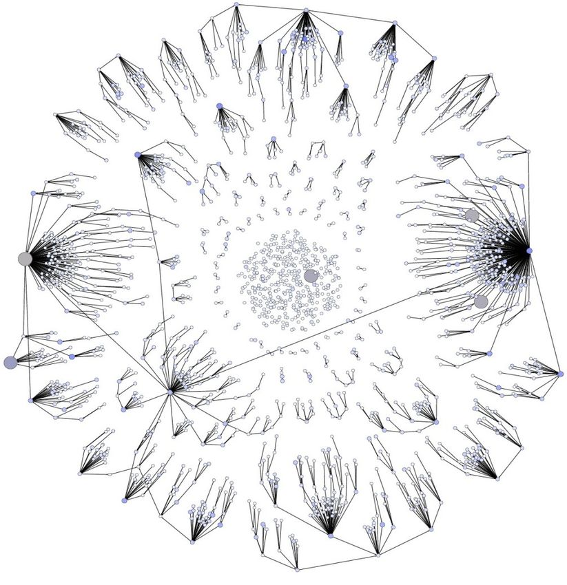
(a) Bigfoot (rumor) (b) Summize (non-rumor)
S̄(t) =S(t) + q(t), Figure 2: Diffusion network examples
2π
q(t) = qa 1 + sin (t + qs ) ,
qp
All other terms are the same as in SpikeM. Figure 2 depicts the diffusion networks of two topics:
Bigfoot and Summize. Nodes represent rumor spreaders,
In the PES model, we add periodic external shock function and edges represent incidents of information diffusion. The
q(t) to the initial shock function S(t), and q(t) has param- figure shows that Bigfoot (rumor) involved a larger fraction
eters qp , qa and qs representing the period, amplitude, and of singletons than Summmize (non-rumor). We could find
the shift of the periodic external shock function, respectively. similar trends in other rumor and non-rumor cases.
When qa = 0, the PES model is reduced to SpikeM, hence From a friendship network, we also extract the largest con-
working as a generalization of the SpikeM model. nected component (LCC). We test the structural properties
For parameter learning, we use Levenberg-Marquard based on three network structure: the friendship network, the
methods to P minimize the sum of the squared errors: LCC of the friendship network, and the diffusion network.
2
D(X, θ) = n (X(n) − ∆B(n)) with a given timseries Table III shows a total of 15 structural features.
X(n). We will show in Section V that these new features
introduced by the PES model turn out to be the most Table III: Structural features.
effective in classifying rumors. Table II displays the temporal Symbols Definition
features in the PES model. Vg Number of Nodes in the friendship network
Eg Number of Links in the friendship network
Table II: Temporal features Dg Density of the friendship network
Cg Clustering Coefficient of the friendship network
Symbols Definition Ig Median in-degree of the friendship network
N Total population of available users Og Median out-degree of the friendship network
β Probability of infection Fl Fraction of nodes in the LCC
nb Starting time of breaking news Vl Number of nodes in the LCC
Sc Strength of external shock at birth (time nb ) El Number of links in the LCC
Background noise Dl Density of nodes in the LCC
pa Strength of interaction periodicity Cl Clustering Coefficient in the LCC
ps Interaction periodicity offset Il Median in-degree in the LCC
qa Strength of external shock Ol Median out-degree in the LCC
qp Periodicity of external shock Sd Fraction of singletons in the diffusion network
qs External shock periodicity offset Fd Fraction of diffusion from low- to high-degree nodes
B. Structural properties C. Linguistic properties.
We define the friendship network as the induced subgraph We utilize a sentiment tool called the Linguistic Inquiry
of the original follower-followee graph induced by those and Word Count (LIWC), which is a transparent text analysis
users who posted at least one related tweets and follow links program that counts words in psychologically meaningful
among them. categories [9]. Its dictionary includes around 4,500 words
Diffusion is defined as follows a topic is diffused from and word stems and the program shows the proportion of
user A to user B, if and only if (1) B follows A on Twitter words that are related to a given sentiment in an input file.
and (2) B posted about a given topic by mentioning the The LIWC provides five major categories and a number of
appropriate keywords only after A did so. In case a user has subcategories in its psychological processes (e.g., social, af-
multiple possible sources, we pick the user who posted about fective, cognitive, perceptual, and biological processes). Full
the topic the latest as the source. Removing all the links over list available at http://www.liwc.net/descriptiontable1.php.
which a diffusion did not occur from the friendship network, We tested whether any of the major or subcategories appear
then yields the diffusion network. dominantly in rumors and non-rumors.Before applying the sentiment tool, we cleaned up the infection rate and often terminating the propagation process.
tweet data by removing usernames, short URLs, as well as As a result, rumors may rely more on the birth of new seeds
emoticons that the tool could not parse. Because sentiment (i.e., new root nodes), who are influenced by external sources
tools require some minimum amount of text as input (e.g., (i.e., external shock). The fact that this temporal pattern is
50 words), we consolidated all the cleaned up tweets into a the most effective predictor for classifying rumors is novel.
single file per topic for analysis. Second, the structural features also had high predictive
power. Among them, the fraction of information flow from
V. RUMOR C LASSIFICATION IN T WITTER
low to high-degree nodes (i.e., diffusion from less influ-
We consider the features on the rumor diffusion patterns ential to more influential people) was the most effective.
of over time (11 temporal features), the shape of the dif- The fraction of singletons (i.e., users whose tweet were
fusion network and the friendship network (15 structural not mentioned or retweeted by others) is also one of the
features), and the language used in the content (65 linguistic recommend classifier, indicating that most of the times the
linguistic features) to classify rumors in Twitter. followers neglect the message. These findings are in tune
A. Feature selection with the attention seeking behavior of rumor initiators [14].
Third, the linguistic features indicated reaction of people
We used random forest and logistic model to quantify
toward rumors. Rumors were significantly less likely to
which features are most informative. For the variable selec-
contain positive affect words (i.e., ‘posemo’ in Table IV than
tion in random forest, we used 2-fold cross-validated pre-
non-rumors (p-= 1.7e−5 ). Also, users are far more likely to
diction with sequentially reduced number of predictors [15]
mention negating words (e.g., no, not, never) in sentence
to find the best number of variables. By this strategy, we
and take a cognitive action (e.g., cause, know) to the rumor
selected 11 variables with the highest importance.Table IV
related content (p = 3.2e−6 ). Also users are more likely to
displays the set of all such significant features determined
take an inferring action (i.e., tentatative) for rumors. This can
from the t-test at 0.05-level (pTable VI: The average performance for each classification Acknowledgement
method: B (baseline with 15 features from [3]), S1 (pro- This research was supported by Basic Science Research
posed in this paper with 11 features), and C (combinaton of Program through the National Research Foundation of Korea
baseline and our proposed method with 27 features) (NRF) funded by the Ministry of Education, Science and
Set Method Accuracy Precision Recall F1 Technology (2011-0012988) and the ICT & Future Planning
B Decision Tree 0.669 0.821 0.717 0.685 (2012R1A1A1014965).
Random Forest 0.747 0.771 0.813 0.762
SVM 0.811 0.891 0.753 0.788 R EFERENCES
S1 Decision Tree 0.791 0.854 0.772 0.780
Random Forest 0.900 0.935 0.892 0.893 [1] G. Allport and L. Postman. The psychology of rumor.
SVM 0.875 0.934 0.838 0.859 Rinehart & Winston, 1947.
C Decision Tree 0.821 0.853 0.843 0.822
Random Forest 0.897 0.923 0.883 0.878 [2] P. Bordia and R. Rosnow. Rumor rest stops on the information
SVM 0.873 0.908 0.873 0.867 highway: Transmission in a computer-mediated rumor chain.
Human Communication Research, 25:163–179, 1998.
[3] C. Castillo, M. Mendoza, and B. Poblete. Information
of recommended features based on random forest (which credibility on twitter. In WWW, 2011.
we call S1 and is composed of 11 significant features
as listed in Table V and logistic regression (which we [4] M. Cha, H. Haddadi, F. Benevenuto, and K. Gummadi.
call S2, composed of 9 features). We also constructed a Measuring User Influence in Twitter: The Million Follower
combined set, C = B ∪ (S1 ∪ S2), with a total of 27 Fallacy. In ICWSM, 2010.
features. We compared the baseline (B) with one of our [5] N. DiFonzo and P. Bordia. Rumor psychology: Social and
features (S1) and the combined set (C), by adopting standard organizational approaches. American Psychological Associ-
three classification algorithms: decision tree, random forest, ation, 2007.
and SVM.Random forest gave marginally better result than
logistic regression in the comparison of S1 and S2. Hence, [6] N. DiFonzo, P. Bordia, and R. Rosnow. Reining in rumors.
Organizational Dynamics, 23:47–62, 1994.
we use S1 as the representative classification method of
our features. For each feature set, we applied 1000 times [7] E. Foster and R. Rosnow. Gossip and network relationships.
of 2-fold cross validation and calculated the average recall, D.C. Kirkpatrick, S. Duck and Foley, M. K. (eds) Relating
precision, and F1 measure. Difficulty: the Processes of Constructing and Managing Dif-
ficult Interaction, 2006.
Table VI displays the results. For each feature set, we
highlight the best performing classification method in bold [8] Y. Matsubara, Y. Sakurai, B. Prakash, L. Li, and C. Faloutsos.
text. For instance, SVM gave the best result for baseline and Rise and fall patterns of information diffusion: Model and
random forest gave the best result for our features. Overall, implications. In KDD, 2012.
the table clearly demonstrates that our features (S1) retain a
[9] J. W. Pennebaker, M. R. Mehl, and K. G. Niederhoffer.
much higher value for every measure compared to baseline. Psychological Aspects of Natural Language Use: Our Words,
The difference between based on the F1 measure is 0.788 Ourselves. Annual Review of Psychology, 54:547–577, 2003.
for baseline and 0.893 for our features. Furthermore, the
combined set (C) does not always give improvement and [10] J. Ratkiewicz, M. Conover, M. Meiss, B. Gonçalves, A. Flam-
sometimes even lead to overfitting, as indicated by the lower mini, and F. Menczer. Detecting and Tracking Political Abuse
in Social Media. In ICWSM, 2011.
value of the F1 measure of C (0.878) compared to that of
S1 (0.893). These results indicate that our original features [11] R. Rosnow. Inside rumor: A personal journey. American
play an important role in rumor classification compared to Psychologist, 46:484–496, 1991.
the best known features that have been studied before.
[12] T. Shibutani. Improvised news: A sociological study of rumor.
Bobbs-Merrill, 1996.
VI. C ONCLUSION
[13] D. Solove. The future of reputation: Gossip, rumor, and
privacy on the Internet. Yale Univ Pr, 2007.
We studied the rumor spreading pattern on Twitter and
tried to classify rumors from non-rumors. Here, three sets [14] C. Sunstein. On Rumours: How Falsehoods Spread, Why We
of features are explored: temporal, structural and linguistic. Believe Them, What Can Be Done. Penguin, 2011.
To extract temporal and structural feature sets, we addressed
[15] V. Svetnik, A. Liaw, C. Tong, and T. Wang. Application
new time series fitting model and network structure. Com- of breimans random forest to modeling structure-activity
bined with a set of linguistic features, our integrated feature relationships of pharmaceutical molecules. Multiple Classifier
set shows a more accurate result of identifying rumors from Systems, pages 334–343, 2004.
other type of information than baseline features.You can also read