Simulation-Based Impact of Connected Vehicles in Platooning Mode on Travel Time, Emissions and Fuel Consumption
←
→
Page content transcription
If your browser does not render page correctly, please read the page content below
Simulation-Based Impact of Connected Vehicles in Platooning Mode on
                                                       Travel Time, Emissions and Fuel Consumption
                                                           Aso Validi Student Member, IEEE, Cristina Olaverri-Monreal Senior Member, IEEE

                                              Abstract— Several approaches have been presented during           simulators and makes it possible to test applications that are
                                           the last decades to reduce carbon pollution from transportation.     additionally based on Vehicle-to-Infrastructure (V2I) or/and
                                           One example is the use of platooning mode. This paper                Vehicle-to-Pedestrian (V2P) communication [8]–[11]. The
                                           considers data obtained from daily trips to investigate the
                                                                                                                3DCoAutoSim simulator is also linked to SUMO (Simula-
arXiv:2105.10894v2 [eess.SY] 26 May 2021

                                           impact of platooning on travel time, emissions of CO2 , CO,
                                           NOx and HC and fuel consumption on a road network in Upper           tion of Urban Mobility) [12] for microscopic road traffic
                                           Austria. For this purpose, we studied fuel combustion-based          simulation and connected to the Robotic Operation System
                                           engines relying on the extension of the 3DCoAutoSim simulation       (ROS) [13].
                                           platform. The obtained results showed that the platooning mode          Additionally, other simulators such as the simulator Ve-
                                           not only increased driving efficiency but also decreased the total
                                           emissions by reducing fuel consumption.                              hicular Network Interface (Veins) [14] uses SUMO and
                                                                                                                provides an extension for evaluation and analysis of pla-
                                                                 I. I NTRODUCTION                               tooning systems from a networking a road traffic perspective
                                                                                                                (Platooning Extension for Veins, PLEXE) [15]. Veins also
                                              According to a report from the Intergovernmental Panel            uses the Objective Modular Network Testbed in C++ (OM-
                                           on Climate Change (IPIC), the transport sector accounts for          NeT++) [16] network simulator. This combination enables
                                           approximately 23% of global CO2 emissions [1]. In 2019               a detailed simulation of wireless communication among
                                           a 28% increase was shown, compared to 1990 levels [2].               vehicles (in particular IEEE 802.11p-based communication)
                                           This development is mainly due to transportation activities          together with realistic mobility patterns.
                                           that result from increased customer demand and consequent               Therefore, we built on PLEXE to extend the vehicular
                                           growth of e-commerce [3]. Current transportation systems             communication capabilities of the 3DCoAutoSim platform
                                           are highly dependent on burning fossil fuels like gasoline and       and connect several delivery vans traveling on the same route
                                           diesel. Therefore, it is crucial to work towards sustainable         via vehicle-to-vehicle communication. As the Traffic Control
                                           transportation through alternatives that reduce fuel consump-        Interface (TraCI) [17] provides access to SUMO through
                                           tion and the emissions of greenhouse gases (GHG) that cause          a Transmission Control Protocol (TCP)-based client/server
                                           the Earth’s atmosphere to warm [2].                                  architecture, we relied on it to link both simulation platforms.
                                              Further research towards a sustainable transport strategy         We then used real data collected from delivery trips of bio-
                                           includes traveling time and origin-destination matrices to           products in Upper Austria and analyzed the effects of driving
                                           improve travel schedules through the analysis of the most            in platooning mode on travel time, GHG emissions and fuel
                                           convenient routes for a specific trip [4]. In this context, a        consumption.
                                           reliable delivery time prediction contributes to eliminating            The remaining parts of this paper are organized as follows:
                                           accessory customer trips to a pick up location or avoiding           the next section describes related work; the section III
                                           additional travel from the side of the delivery company to           presents the methodology adopted to link the different
                                           return the goods to the sender [5].                                  modular components within the 3DCoAutoSim simulation
                                              There exist other technology-based approaches that per-           platform and to perform the comparative analyses; the results
                                           tain to the field of Intelligent Transportation Systems (ITS)        from the analyses of the defined scenarios are presented in
                                           that can curtail global temperature increases. For example,          section IV; and the section V concludes the work and outlines
                                           autonomous delivery robots can overcome challenges related           future research.
                                           to navigation in an urban environment, including parking and
                                           its effect on fuel consumption, fuel costs and CO2 emissions                             II. R ELATED W ORK
                                           [3].                                                                    There has been a marked increase in research works that
                                              The 3DCoAutoSim simulation platform was originally                target decreased dependence on fossil fuels in the transporta-
                                           implemented to mimic Vehicle-to-Vehicle (V2V) [6] commu-             tion sector.
                                           nication from a driver-centric perspective [7] and has been             We review and summarize in this section platooning-
                                           continuously extended to include automated capabilities and          related published works, highlighting the contribution of our
                                           reproduce cooperative Advanced Driving Assistance Systems            work to the state of the art.
                                           (ADAS). It uses vehicular data connection among multiple                By relying on the Scania Truck And Road Simulation
                                                                                                                (STARS) [18] simulated environment the authors in [19] in-
                                             Johannes  Kepler    University   Linz,         Austria; Chair
                                           Sustainable Transport    Logistics   4.0.         {aso.validi,       vestigated the effect of heavy duty vehicle (HDV) platooning
                                           cristina.olaverri-monreal}@jku.at                                    on fuel reduction. Results from the study showed a maximum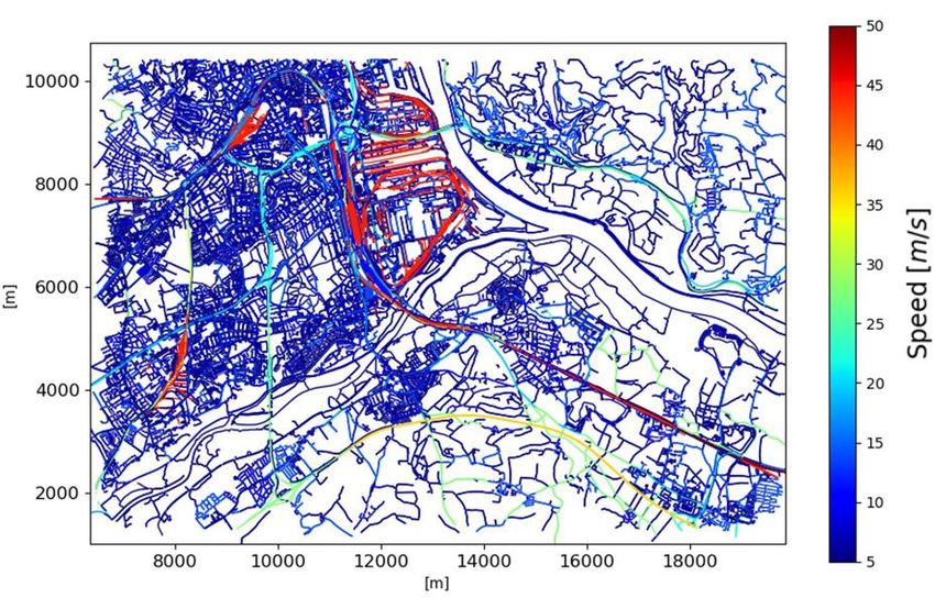
fuel reduction of 4.7–7.7% at a speed of 70 km/h that was
dependent on the time gap and the number of vehicles in
the platoon. The authors reported vehicle weight to be an
additional influential factor on the platooning system, with
the fuel reduction of 3.8–7.4% when the lead vehicle was 10
tonnes lighter in contrast to a 4.3–6.9% fuel reduction when
the lead vehicle was 10 tonnes heavier.
   In further studies relying on the simulation of urban
mobility SUMO, the effects of platooning on the generation
of emissions were investigated in different networks by
applying Cooperative Adaptive Cruise Control (CACC) [20],
[21]. The authors relied on the combination of OMNet++ and
Veins. The road and network simulation tools assumed the
HBEFA3 emission model in all vehicles, according to the
classification in the Handbook Emission Factors for Road
Transport (HBEFA) [22]. The studies focused on exploring
different penetration rates of CACC varying from 0-100% in
25% increments in two scenarios with intersections regulated
by fixed and adaptive traffic light control. The maximum
GHG emission reduction reported in the study was 20% [20].
   A two-layer Control Look-Ahead Control (CLAC) archi-
tecture for fuel-efficient and safe heavy-duty vehicle pla-
tooning was proposed and simulated in [23] to obtain road
information and real time control of the vehicles. Through           Fig. 1. Overview of the modular components within the “3DCoAutoSim”
Dynamic Programming (DP), the optimal speed of the pla-              simulation framework
toon for maximum fuel efficiency was estimated. For real-                                     TABLE I
time control, a predictive control framework was considered.             PARAMETERS VALUES TO SETUP THE SIMULATION SCENARIOS
The approach resulted in a maximum fuel savings of 12%
for following vehicles in the platoon.                                                  Parameters             Value
   This represents a selection of the variety of methodologies                                min          5m/s(18km/h)
                                                                                     Speed
developed and adopted to investigate platooning-related met-                                  max          20m/s(72km/h)

rics that pertain to traffic flow, such as fuel efficiency, travel                   Acceleration (max)       2.5m/s2
                                                                                     Delivery van weight      3500kg
time, and pollutant emissions. However, studies that use data
                                                                                     Delivery van length       5.94m
generated from real road trips are very scarce. Therefore,
we contribute with this work to the gap in the body of
knowledge by performing research on platooning using a
simulation platform with real data sets collected from real
trips in Austria.                                                    we compared the data obtained from three delivery vans
                                                                     under the following two scenarios:
                     III. M ETHODOLOGY                                 1) Connected in platooning mode, the vehicles in
   As previously mentioned, we extend in this work the                    this scenario being labeled as: Leader.Delivery-
“3DCoAutoSim” simulation platform with SUMO and the                       Van.1 (LDV1), Follower.Delivery-Van.2 (FDV2) and
vehicular communication capabilities that are enabled by                  Follower.Delivery-Van.3 (FDV3).
the Veins network interface and the network simulation                 2) Not connected, the vehicles in this scenario being la-
OMNet++ to simulate a IEEE 802.11p wireless network-                      beled as: Delivery-Van.1 (DV1), Delivery-Van.2 (DV2)
based communication and to design and simulate longitu-                   and Delivery-Van.3 (DV3).
dinal controllers. An overview of the linked components                 The relevant parameters to set up the simulation that were
that compose the “3DCoAutoSim” simulation framework is               common to both scenarios are presented in Table I. The input
presented in Figure 1. The 3D visualization in the simulator         that we selected for the gap size parameter in the platooning
is based on Unity, which makes it possible to simulate a             mode was of 5m [15]. The value corresponded to an average
variety of controlled driving environments through realistic         speed of 70.2km/h and 71.28km/h.
car controller assets. UNITY, ROS and SUMO are connected                The considered route in the scenarios is based on the real
by relying on the rosbridge package [24] and the TraCI               GPS data gathered from 12 trips (morning trips at around
interface.                                                           11:00 am) with an average travel time and speed of 20min
   To validate the implemented approach, we analyzed the             and 20m/s (72km/h) respectively. The trips were performed
effect of platooning on the dependent variables travel time,         by the Achleitner Biohof GmbH (Achleitner Organic farm)
total emissions and vehicular fuel consumption. To do this,          in the itinerary around Linz in Upper Austria, which are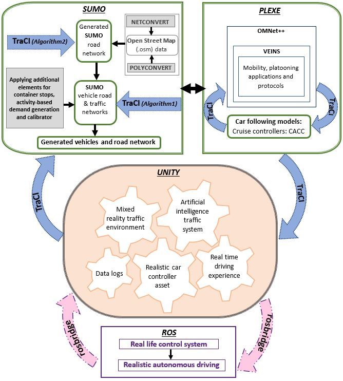
TABLE II
C OLLECTED TRIP DATA
Parameters Explanation
Day day of tracking (format: T:name of the day)
Date date of tracking (format: Y:year, M:month, D:day)
Time time of tracking in every second (format: H:hour, M:minute, S:second)
Latitude n/s north–south geographic coordinate
Longitude e/w east–west geographic coordinate
Height elevation above sea level (unit: meter)
Speed speed of vehicle at every second (unit: kilometer)
Heading compass direction (unit: degree)
VOX recorded voice messages
Fig. 3. Visualization of the maximum speed limit in m/s on different routes
in the simulated road network
to import and convert the road network. To interpret the
relevant geometrical shapes from the OSM data, an addi-
tional typemap-file [27] was utilized, which converted the
data to be visualized in the SUMO Graphical User Interface
(GUI) through POLYCONVERT [28]. We also applied the
NETEDIT application [29] for updating the traffic lights and
editing the road network in terms of size and type. In order
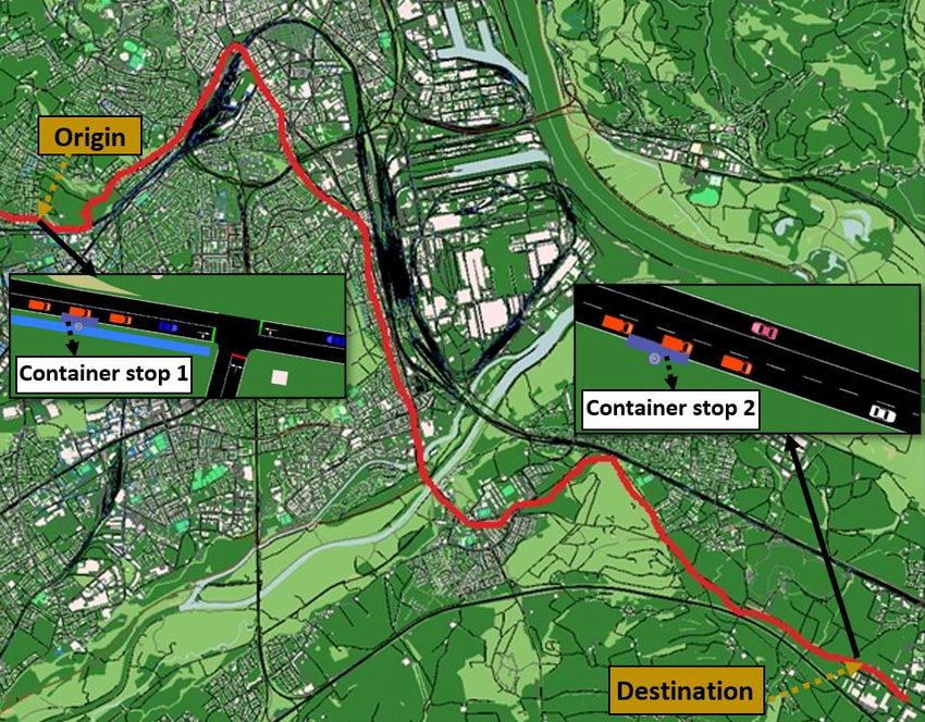
Fig. 2. Visualization of the collected travel data showing the driven route to have a better overview on the network, we additionally
(14km) and the pick up and delivery van stops
visualized the maximum speed limit on different routes in
the road network (Figure 3). To replicate reality-close traffic
Algorithm 1: Applying TraCI for generating the route conditions we generated the network demand by relying on
files and vehicles in the different scenarios statistics from the city of Linz and applying activity-based
input : Road Network, r;
output: Route file, rou;
demand generation using Iterative Assignment (Dynamic
define : Number of vehicles i, Number of time steps n, User Equilibrium) [30] in 3 iterations. After these steps, we
Vehicle types; platooningvType, vanvType implemented the vType attribute to characterize the vehicle
1 Function RoutVehGenerate(): types from the traffic demand. Each individual vehicle in
2 random.seed(s) the simulation was defined by a unique identifier, departure
3 N←n
output: .rou.xml (vType, edges, vehid )
time and planned route. We additionally adopted TraCI, to
4 be able to retrieve the values of the simulated objects and
5 vehNr ← 0 to manipulate their behavior in real time [17]. Finally, we
6 for i in range(N) do calibrated the traffic flow in the simulation [31].
7 if random.uniform(0,1) < each of the three
delivery vans: then Algorithm 1 describes the process for generating the route
8 write output’< generating the vehicle types files and the traffic demand using TraCI, which used the
with different attributes/ >’ format (i,vehNr), relevant files in the road network (.osm and .net) as input
file = routes
9 vehNr + = 1 information. It starts by generating the defined vType and
10 end the routes with the related edges on the .rou.xml file. This is
11 end then followed by the creation of the vehicles based on their
12 End Function specified probabilities for each of the routes on the .rou file.
To generate the different types of vehicles, the algorithm
randomly assigns numbers to vehicle IDs. The route file
illustrated in the road network in Figure 2 after the data generation follows the defined format by generating all the
processing and cleaning procedure. The detailed collected related attributes, such as type, route ID and departure time.
information about the daily trips is presented in Table II. This vehicle creation and definition follows the specified
format by generating all the related attributes, such as type,
A. Traffic simulation implementation route ID and departure time. To complete all the relevant
To generate the traffic network the map data was im- situations in the simulation, additional elements such as
ported from Open Street Map (OSM) [25] to SUMO. The “container stops” [32] were defined to mimic loading or
SUMO application NETCONVERT [26] was then executed delivery locations.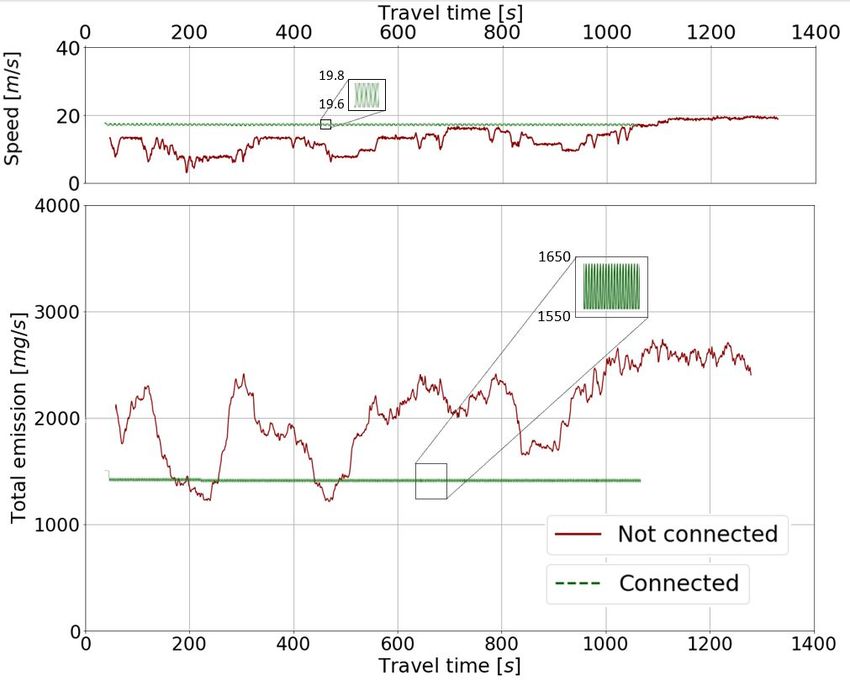
Algorithm 2: Applying TraCI for collecting and calcu-
  lating emissions
    input : Road Network, r;
    output: Emission file; (GHG)
    define : Emission class; ec, Number of vehicles i, Number
             of time steps n, Vehicle types
 1 Function GetVehEmission(vehid ):
 2      co2 ← traci.getCO2Emission (vehid )
 3      co ← traci.getCOEmission (vehid )
 4      nox ← traci.getNOxEmission (vehid )
 5      hc ← traci.getHCEmission (vehid )
 6      return EmissionSense
 7 End Function
 8 Function VehEMISSIONcal():
 9      for vehid in traci.getIDList(): do                       Fig. 4. Travel time resulting from comparing the simulated delivery vans
                                                                 in “connected” vs “not connected” mode
10           vehpos ← traci.getPosition (vehid )
11           vehicle ← Vehicle (vehid , vehpos )
12           vehicle.emissions ← calvehemissions (vehid )
13           vehicles.append(vehicle)
14           return vehiclesemissions
15      end
16 End Function

B. Vehicle connection definition

   We generated the platooning simulation by modifying the
behavior of the vehicles by accessing the related node in
OMNeT++, the new behavior being applied to the driven
routes. In the OMNeT++ configuring models (.ned and
.ini files), we adopted the SimplePlatooningBeaconing class
[33], which extends the base protocol [34] for the use
of communication protocols. This implemented class is a
classic periodic beaconing protocol which sends a beacon
every x milliseconds. Furthermore, in order to generate a        Fig. 5.   Speed profile (top) and average total emissions (bottom) in
                                                                 “connected” vs “not connected” mode
set of real world simulations with human driven vehicles in
combination with platooning, we adopted the HumanInter-
feringProtocol [35] application. This class transmits periodic   C. Emissions calculation
beacons from human-driven vehicles and makes it possible
to generate interfering network traffic. This approach will be      To study the total emissions and fuel consumption, we
part of future studies with real drivers.                        relied on the “HBEFA3/LDV-D-(EU6)” emission class that
   The implementation of the simulation for the driven routes    includes the weight and length of the delivery vehicles
from which the data was acquired requires a high computa-        used [22]. The calculation of the emissions data is expressed
tional capacity that is intensified through the integration of   through Algorithm 2 using retrievable vehicle variables
Veins to link OMNeT++ and SUMO through TraCI. Hence,             through TraCI. The algorithm uses as input the main road
to run the entire network simulation as smoothly as possible,    network data files (.rou.xml and .add.xml) with the defined
we generated a few numbers of SUMO vehicles that were not        emission class and the vehicle types. It then detects and
defined as OMNeT++ nodes and did not have communication          stores the GHG produced by the vehicles (CO2 , CO, N Ox,
capabilities. For managing the platoon traffic in the road       HC) in each time step. Based on the vehicle position, the
network, we applied the nCars and platoonSize configuration      algorithm classifies the gathered data and finally calculates
parameters from the PlatoonsTrafficManager [36] class. The       the emissions for each of the vehicles.
parameters represent the total number of vehicles and the
number of vehicles per platoon, respectively.                    D. Comparative analysis description
   To this end, we adopted sinusoidal mode of speed in pla-         To investigate the potential and beneficial effects of driving
toon with oscillation frequency of 0.2Hz [15]. We also took      in platooning mode, we conducted a set of comparative
advantage of the configuration parameters of omnetpp.ini         analyses of the use cases defined in section III. To this
namely ’manager.moduleType’ and ’manager.moduleName’             end, we analyzed the following key metrics: travel time,
by setting ’vtypehuman’ to zero (vtypehuman is the param-        total emissions and fuel consumption obtained from the
eter definition key for the defined vehicles in PLEXE).          simulation. The total emission analysis was performed by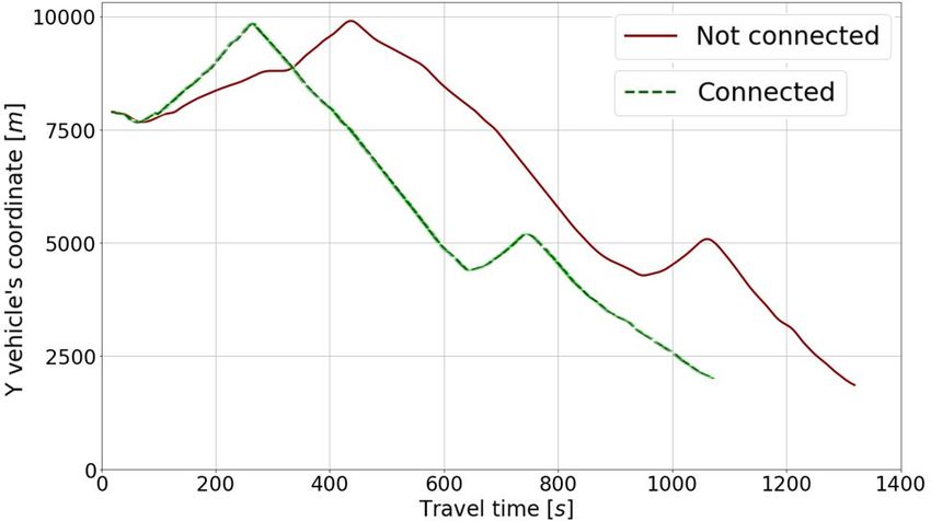
TABLE III
                                                                                 E MITTED POLLUTANT VALUES DURING THE STUDIED TRIPS

                                                                                                          Co2               N Ox            CO             HC
                                                                                                       (cumulated)       (cumulated)    (cumulated)     (cumulated)
                                                                                                          mg/s              mg/s           mg/s            mg/s
                                                                                           LDV1     1623.25             1.85           0.196           0.006
                                                                                                                               SUM=            SUM=            SUM=
                                                                          Connected        FDV2     1544.45   SUM=      1.67           0.190           0.005
                                                                                                                               4.94            0.573           0.014
                                                                                           FDV3     1474.34   4642.04   1.42           0.187           0.003
Fig. 6.    Speed and acceleration effects on CO2 emissions in “not                         DV1      1991.75             3.41           0.986           0.037
                                                                                                              SUM=             SUM=            SUM=            SUM=
connected” mode                                                           Not connected    DV2      1883.48
                                                                                                              5673.21
                                                                                                                        3.36
                                                                                                                               9.99
                                                                                                                                       0.871
                                                                                                                                               2.699
                                                                                                                                                       0.034
                                                                                                                                                               0.094
                                                                                           DV3      1797,98             3.22           0.842           0.023

Fig. 7. Speed and acceleration effects on CO2 emissions in “connected”
platooning mode

calculating the emission values of the following pollutants
CO2 , CO, NOx and HC for each use case.
                          IV. R ESULTS
A. Travel time
                                                                                 Fig. 8.     Comparison between cumulative fuel consumption
   The differences in the speed of the “connected” compared
to the “not connected” vehicles (Figure 5 top) resulted in a                                               TABLE IV
reduced travel time of 22.38% (see Figure 4). The delivery                                 K EY M ETRICS IN THE S TUDIED S CENARIOS
vans that were not connected needed 1385 seconds each to
drive through the route visualized in Figure 2, starting from                                           Travel Time
                                                                                                                           Total Emissions      Fuel Consumption
                                                                                                                             (cumulated)           (cumulated)
the “container stop 1”, defined as origin, to the destination                                                s
                                                                                                                                mg/s                  ml/s
in “container stop 2”.                                                                       LDV1                         1625.30
                                                                                                                                    SUM =
                                                                                                                                                0.597
                                                                                                                                                        SUM =
                                                                          Connected          FDV2             1075        1546.31               0.557
                                                                                                                                    4647.57             1.651
B. Total emissions                                                                           FDV3                         1475.95               0.497
                                                                                             DV1                          1996.18               0.786
                                                                                                                                    SUM =               SUM =
   The average emission values obtained from simulating                   No connected       DV2              1385        1887.74               0.772
                                                                                                                                    5685.99             2.301
“connected” and “not connected” scenarios and their related                                  DV3                          1802.06               0.743

speed profiles are plotted in Figure 5 bottom and top respec-
tively. In the delivery vans that were not driving in platooning
mode, the fluctuations in the total emissions reflect the                vans that are not connected. As it can be seen, acceleration
acceleration and deceleration of the vans throughout the                 has a high impact on CO2 emissions. The highest value
total trip. The driving patterns variation was related to the            of CO2 is emitted at a speed of 19.5m/s (70.2km/h)
topology of the road. The higher value of the total emissions            with an acceleration value of approximately 2.5m/s2 . Fig 7
in “not connected” at the end of the trip (at 1100 s) was due            shows the relationship between CO2 emissions, speed, and
to the higher road speed limit (see speeds in Figure 3).                 acceleration of the delivery vans in platooning mode. The
   In the connected platooning mode, all the three vans                  CO2 emissions are, with a value of 1547.34mg/s, lower than
formed the platoon within a few seconds of the start of                  those in the “not connected” mode (1891.07mg/s), due to
the trip, and maintained a steady average speed of 19.8m/s               low variability of the speed and acceleration metrics (accel-
(71.28km/h). The average value of the generated emissions                eration values between 2.2 and 2.4 m/s2 and speed values
is represented by a flat line with a subtle level of sinusoidal          between 19.6m/s (70.56km/h) and 19.8m/s (72km/h).
acceleration and deceleration in speed (see section III-B),              The detailed pollutant values of the individual delivery vans
which are characteristics of driving in platooning mode                  for each scenario are presented in Table III.
(zoomed scale rectangular of Figure 5). The values for the
total GHG emissions in each of the individual delivery vans              C. Fuel consumption
are represented in Table IV.                                                Cumulative fuel consumption results for “connected” and
   As carbon dioxide (CO2 ) is one of the main GHG that                  “not connected” are presented in Figure 8, the graphic
contributes to global warming, we additionally performed                 showing a 28.25% reduction of fuel consumption when the
a complementary analysis of the generated CO2 emissions                  delivery vans are connected and build a platoon. A summary
(Figure 6 and Figure 7). Figure 6 shows the relationship                 of all the obtained values for “travel time”, “total emissions”,
between CO2 emissions, speed, and acceleration in delivery               and “fuel consumption” are presented in Table IV.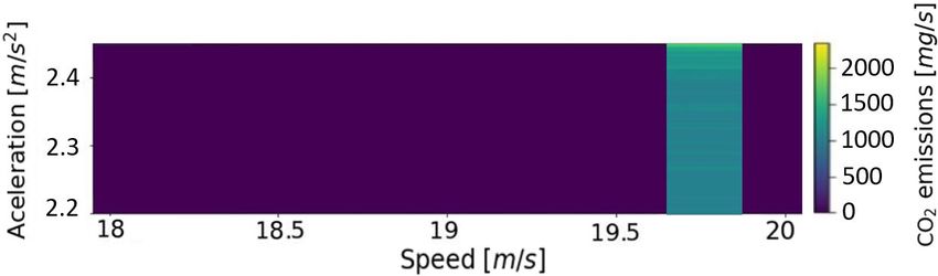
V. C ONCLUSION AND F UTURE W ORK                                   [11] L. Artal-Villa and C. Olaverri-Monreal, “Vehicle-Pedestrian Inter-
                                                                                     action in SUMO and Unity3D,” in Proceedings WorldCIST 2019.
   To increase the efficiency of transportation, a variety of                        Springer International Publishing AG, Cham, Switzerland, 2019, p. .
alternatives has been investigated in the past few decades.                     [12] M. Behrisch, L. Bieker, J. Erdmann, and D. Krajzewicz, “Sumo–
Vehicular connectivity and platooning are among the most                             simulation of urban mobility: an overview,” in Proceedings of SIMUL
                                                                                     2011, The Third International Conference on Advances in System
promising technological ITS solutions, as they reduce fuel                           Simulation. ThinkMind, 2011.
consumption and the amount of generated GHG. In this                            [13] M. Quigley, K. Conley, B. Gerkey, J. Faust, T. Foote, J. Leibs, and
paper we presented a microscopic simulation-based method                             A. Ng, “Ros: an open-source robot operating system. icra workshop
                                                                                     on open source software (vol. 3, no. 3.2),” 2009.
to investigate the impact of platooning on travel time, total                   [14] C. Sommer, R. German, and F. Dressler, “Bidirectionally Coupled
emissions, and fuel consumption using fuel combustion                                Network and Road Traffic Simulation for Improved IVC Analysis,”
delivery vans. Based on the results obtained, we conclude                            IEEE Transactions on Mobile Computing (TMC), vol. 10, no. 1, pp.
                                                                                     3–15, January 2011.
that the implemented approach is a feasible solution to in-                     [15] M. Segata, S. Joerer, B. Bloessl, C. Sommer, F. Dressler, and R. L.
vestigate the effect of platooning on relevant global warming                        Cigno, “Plexe: A platooning extension for veins,” in 2014 IEEE
parameters such as travel time, fuel consumption and the                             Vehicular Networking Conference (VNC). IEEE, 2014, pp. 53–60.
                                                                                [16] “OMNeT++ Discrete Event Simulator.” [Online]. Available: https:
generated emissions from fuel combustion vehicles. Further                           //omnetpp.org/
work in this area will be pursued to collect data involving                     [17] “Traffic Conrol Interface.” [Online]. Available: https://sumo.dlr.de/
drivers and electric vehicles in an urban area.                                      docs/TraCI.html
                                                                                [18] “Heavy truck modeling for fuel consumption. Simulations and
                     ACKNOWLEDGMENT                                                  measurements (Thesis/Dissertation) — ETDEWEB.” [Online].
                                                                                     Available: https://www.osti.gov/etdeweb/biblio/20243785
   This work was supported by the FFG project “Zero                             [19] A. Al Alam, A. Gattami, and K. H. Johansson, “An experimental
Emission Roll Out Cold Chain Distribution 877493” and                                study on the fuel reduction potential of heavy duty vehicle platooning,”
                                                                                     in 13th International IEEE Conference on Intelligent Transportation
the Austrian Ministry for Climate Action, Environment, En-                           Systems. IEEE, 2010, pp. 306–311.
ergy, Mobility, Innovation and Technology (BMK) Endowed                         [20] İ. G. Erdağı, M. A. Silgu, and H. B. Çelikoğlu, “Emission effects of
Professorship for Sustainable Transport Logistics 4.0., IAV                          cooperative adaptive cruise control: a simulation case using sumo,”
                                                                                     EPiC Ser. Comput., vol. 62, pp. 92–100, 2019.
France S.A.S.U., IAV GmbH, Austrian Post AG and the UAS                         [21] M. A. Silgu, İ. G. Erdağı, and H. B. Çelikoğlu, “Network-wide
Technikum Wien.                                                                      emission effects of cooperative adaptive cruise control with signal
                                                                                     control at intersections,” Transportation Research Procedia, vol. 47,
                             R EFERENCES                                             pp. 545–552, 2020.
                                                                                [22] “The Handbook Emission Factors for Road Transport (HBEFA) .”
 [1] O. Edenhofer, Y. Sokona, J. C. Minx, K. Seyboth, I. Baum, S. Brunner,           [Online]. Available: https://www.hbefa.net/d/documents/HBEFA3-3
     S. Schlömer, and T. Zwickel, “Report of the Intergovernmental Panel            TUG finalreport 01062016.pdf
     on Climate Change Edited by,” Tech. Rep., 2014. [Online]. Available:       [23] V. Turri, B. Besselink, and K. H. Johansson, “Cooperative Look-Ahead
     www.ipcc.ch                                                                     Control for Fuel-Efficient and Safe Heavy-Duty Vehicle Platooning,”
 [2] O. Pribyl, R. Blokpoel, and M. Matowicki, “Addressing eu climate                IEEE Transactions on Control Systems Technology, vol. 25, no. 1, pp.
     targets: Reducing co2 emissions using cooperative and automated ve-             12–28, 2017.
     hicles,” Transportation Research Part D: Transport and Environment,        [24] “Ros bridge lib, GitHub Repository.” [Online]. Available: https:
     vol. 86, p. 102437, 2020.                                                       //github.com/MathiasCiarlo/ROSBridgeLib
 [3] Y. Liu, G. Novotny, N. Smirnov, W. Morales-Alvarez, and C. Olaverri-       [25] “OpenStreetMap .” [Online]. Available: https://www.openstreetmap.
     Monreal, “Mobile Delivery Robots: Mixed Reality-Based Simulation                org/#map=8/47.714/13.349
     Relying on ROS and Unity 3D,” 2020.                                        [26] “Nnetconvert-sumo documentation.” [Online]. Available: https://sumo.
 [4] J. Gonçalves, J. S. Goncalves, R. J. Rossetti, and C. Olaverri-Monreal,        dlr.de/docs/netconvert.html
     “Smartphone sensor platform to study traffic conditions and assess         [27] “SUMO Geometrical Shapes.” [Online]. Available: https://github.com/
     driving performance,” in 17th International IEEE Conference on                  eclipse/sumo/blob/master/data/typemap/osmPolyconvert.typ.xml
     Intelligent Transportation Systems (ITSC). IEEE, 2014, pp. 2596–           [28] “polyconvert-SUMO Documentation.” [Online]. Available: https:
     2601.                                                                           //sumo.dlr.de/docs/polyconvert.html
 [5] J. Khiari and C. Olaverri-Monreal, “Boosting algorithms for delivery       [29] “netedit - SUMO Documentation.” [Online]. Available: https:
     time prediction in transportation logistics,” in 2020 International             //sumo.dlr.de/docs/netedit.html
     Conference on Data Mining Workshops (ICDMW), 2020, pp. 251–                [30] “Iterative Assignment (Dynamic User Equilibrium).” [On-
     258.                                                                            line]. Available: https://sumo.dlr.de/docs/Demand/Dynamic User
 [6] F. Michaeler and C. Olaverri-Monreal, “3d driving simulator with                Assignment.html
     vanet capabilities to assess cooperative systems: 3dsimvanet,” in 2017     [31] “Calibrator.” [Online]. Available: https://sumo.dlr.de/docs/Simulation/
     IEEE Intelligent Vehicles Symposium (IV). IEEE, 2017, pp. 999–1004.             Calibrator.html
 [7] C. Biurrun, L. Serrano-Arriezu, and C. Olaverri-Monreal, “Micro-           [32] “Specification/logistics-sumo documentation.” [Online]. Available:
     scopic driver-centric simulator: Linking unity3d and sumo,” in World            https://omnetpp.org/
     Conference on Information Systems and Technologies. Springer, 2017,        [33] “PlEXE-Protocols.”         [Online].      Available:      https://github.
     pp. 851–860.                                                                    com/michele-segata/plexe-veins/blob/master/src/plexe/protocols/
 [8] A. Hussein, A. Dı́az-Álvarez, J. M. Armingol, and C. Olaverri-                 SimplePlatooningBeaconing.cc
     Monreal, “3DCoAutoSim: Simulator for cooperative ADAS and auto-            [34] “PlEXE-Protocols.”         [Online].      Available:      https://github.
     mated vehicles,” in 2018 21st International Conference on Intelligent           com/michele-segata/plexe-veins/blob/master/src/plexe/protocols/
     Transportation Systems (ITSC). IEEE, 2018, pp. 3014–3019.                       BaseProtocol.cc
 [9] C. Olaverri-Monreal, J. Errea-Moreno, and A. Diaz-Alvarez, “Imple-         [35] “PlEXE-Protocols.”         [Online].      Available:      https://github.
     mentation and Evaluation of a Traffic Light Assistance system in a              com/michele-segata/plexe-veins/blob/master/src/plexe/protocols/
     Simulation Framework based on V2I Communication,” Journal of                    HumanInterferingProtocol.cc
     Advanced Transportation, 2018.                                             [36] “PlEXE-PlatoonTraffic         Manager.”        [Online].      Available:
[10] C. Olaverri-Monreal, J. Errea-Moreno, A. Dı́az-Álvarez, C. Biurrun-            https://github.com/michele-segata/plexe-veins/blob/master/src/plexe/
     Quel, L. Serrano-Arriezu, and M. Kuba, “Connection of the SUMO                  traffic/PlatoonsTrafficManager.cc
     Microscopic Traffic Simulator and the Unity 3D Game Engine to
     Evaluate V2X Communication-Based Systems,” Sensors, vol. 18,
     no. 12, p. 4399, 2018.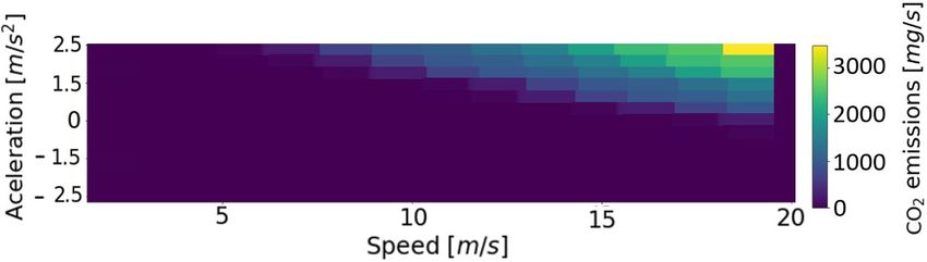
You can also read