Hysteresis without Hope: investigating unemployment persistence in South Africa
←
→
Page content transcription
If your browser does not render page correctly, please read the page content below
Munich Personal RePEc Archive

Hysteresis without Hope: investigating
unemployment persistence in South
Africa

Dadam, Vincent and Viegi, Nicola

University of Pretoria, University of Pretoria and ERSA

31 May 2021

Online at https://mpra.ub.uni-muenchen.de/108129/
MPRA Paper No. 108129, posted 07 Jun 2021 10:19 UTC
Hysteresis without Hope: Investigating Unemployment
                              Persistence in South Africa

                              Vincent Dadam∗                Nicola Viegi†

                                               May 2021

                                               Abstract

          This paper investigates hysteresis in South Africa’s unemployment. First we test the
      presence of hysteresis in unemployment both by traditional stationarity tests and by us-
      ing non-linear transformation methods to identify two further characteristics of hysteresis,
      namely remanence and selective memory. In the second part of the paper we estimate a
      simple insider-outsider model using a Bayesian VAR methodology to identify the shocks
      driving the unemployment dynamics. The main finding is that shocks to nominal wages
      and mark-up shocks as the main drivers of unemployment. Demand shocks do not play
      a dominant role. These results point to the difficulty of absorbing the current level of
      unemployment without significant positive shocks in market structure and wage setting
      behaviour. The strong hysteresis present in the data shows that this excessive level of un-
      employment can become ”equilibrium”: the South African labour market presents features
      of the worst kind of hysteresis, a hysteresis without ”hope”.

∗
    Corresponding author, University of Pretoria, vincent.dadam@up.ac.za
†
    University of Pretoria and Economics Research Southern Africa (ERSA), nicola.viegi@up.ac.za

                                                    1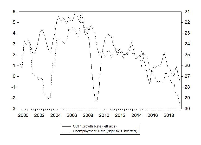
Contents

1 Introduction                                                                                      3

2 Hysteresis in unemployment: definition and evidence                                              4

3 Hysteresis in unemployment: causes and consequences                                              10
  3.1   The model . . . . . . . . . . . . . . . . . . . . . . . . . . . . . . . . . . . . . . .    10
  3.2   Data and Estimation . . . . . . . . . . . . . . . . . . . . . . . . . . . . . . . . .      12
  3.3   Estimation analysis . . . . . . . . . . . . . . . . . . . . . . . . . . . . . . . . . .    13
        3.3.1   Baseline scenario . . . . . . . . . . . . . . . . . . . . . . . . . . . . . . .    13
        3.3.2   Experimental scenarios     . . . . . . . . . . . . . . . . . . . . . . . . . . .   16

4 Conclusion                                                                                       21

                                                2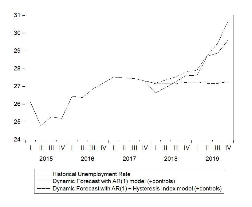
1    Introduction

Unemployment rate in South Africa has a specific dynamics: the rate has been on an upward
trend for the last 10 years, going from 21.1% just before the global financial crisis at the end of
2007 to 29.6% just before the Covid-19 epidemic at the end of 2019. The pattern of unemploy-
ment follows quite closely that of GDP growth, in the 2000-2019 period. Figure 1 shows this
correlation, especially after the global financial crisis when growth and unemployment enter
on a negative trend. This paper studies these patterns and wants to shed some light on what
is driving this double negative trends.

               Figure 1: South Africa Unemployment - GDP Growth 2000-2019

    The first objective of the paper is to identify if the data show the presence of hysteresis
in South Africa unemployment. Hysteresis refers to the fact that a rise in the unemploy-
ment rate following a shock leads to an increase in the underlying equilibrium unemployment
(O’Shaughnessy, 2011). This has fundamental implications for monetary policy because any
subsequent increase in the demand of labour will generate inflationary wage and prices in-
creases before unemployment returns to the pre-shock level. It has also implication for the

                                                3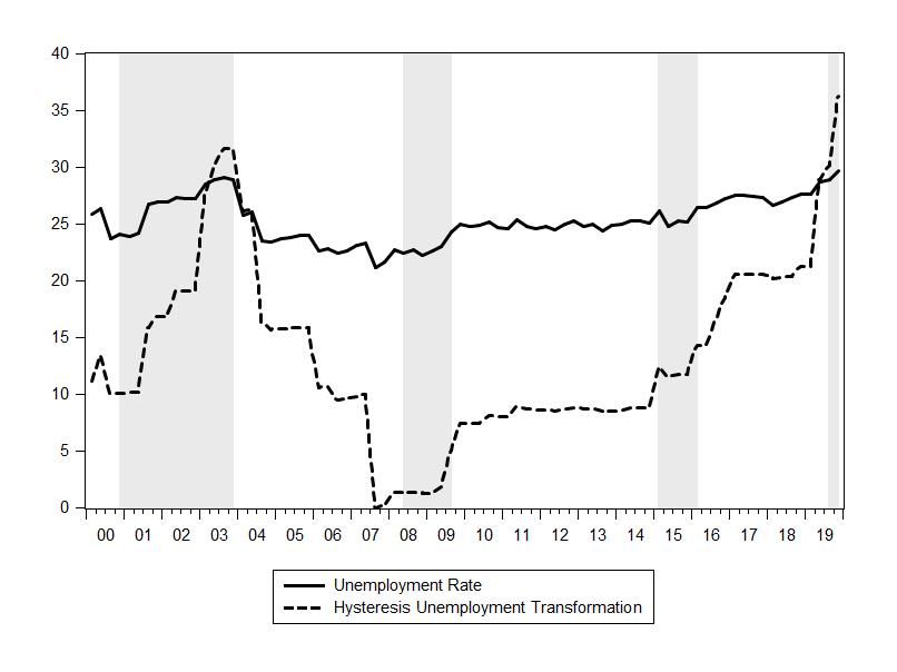
model used for monetary policy as a Phillips curve specification of the relation between infla-
tion and output gap would be wide off the mark.
    Once we have determined that unemployment in South Africa is characterized by strong
hysteresis, we use Bayesian VAR to identify what are the causes of this hysteresis. In particular
we focus on three main determinants: shocks to nominal wages, following Blanchard and Summers
(1987), shocks to mark-up by firms (Gambetti and Pistoresi, 2004) and shocks to the terms of
trade through the exchange rate as a proxy for changes in costs of intermediate and investment
goods affecting firms’ decisions (Darby, Hallett, Ireland, and Piscitelli, 1999).
    The idea of hysteresis in economics was introduced by Blanchard and Summers (1987) and
has found new life after the global financial crisis to explain the persistence of economic stag-
nation when monetary policy is at the zero lower bound (Galı́, 2015, 2020; Garga and Singh,
2021). This study follows the trend by applying the concept to the South African context.
The rest of the paper is therefore set up as follows. Section 2 defines the hysteresis concept
and tests for its evidence in the South African unemployment series. Section 3 is an investi-
gation of the causes and consequences of hysteresis in unemployment in which a simple model
of insiders-outsiders dynamics with hysteresis is set up. The model is later estimated using
Bayesian VAR, with the results discussed in the same section. Section 4 concludes.

2    Hysteresis in unemployment: definition and evidence

The term hysteresis is widely used in economics to cover different concept of persistence in
economic dynamics. For example, Galı́ (2020) interprets hysteresis as a long lasting deviation
of unemployment from a ”flexible wages” underlying natural rate of unemployment, while
Garga and Singh (2021) interpret hysteresis as a permanent change in potential output, i.e. a
unit root in the underlying equilibrium values. Both approaches try to mimic the unit root in
unemployment or economic growth observed for many countries.
    The first test for hysteresis is then a test of memory of the series, i.e. a simple unit root
test. In Table 1 we report the results of Augmented Dickey-Fuller (ADF) and Phillips-Perron
tests for unit root on the South African unemployment series. The tests cannot reject the
hypothesis of a unit root at any confidence level, a result confirmed with any other unit root
test available.

                                                4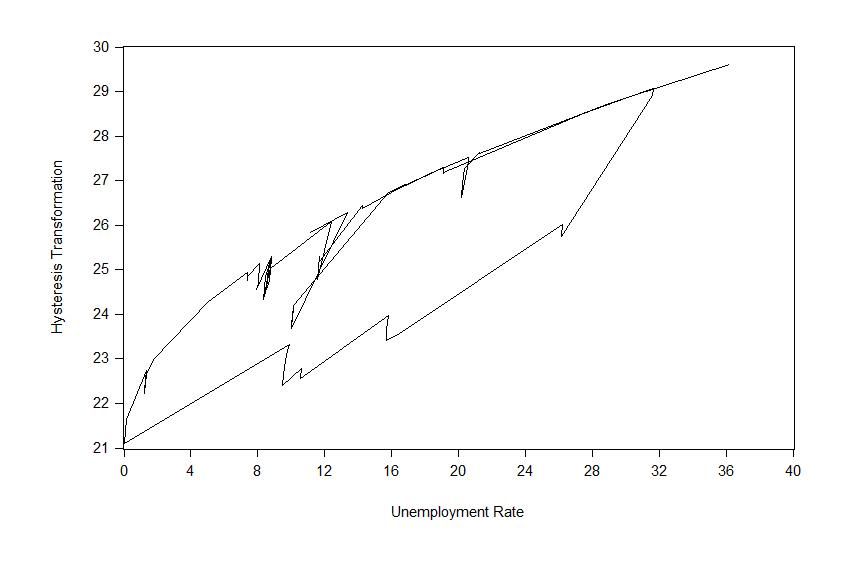
Table 1: Unit Root Tests on South Africa Unemployment 2000q1-2019q4

        Null Hypothesis: Unemployment has a unit root            Adj. t-Stat      Prob.*

        Augmented Dickey-Fuller test statistic                   −1.384906        0.5856
        Phillips-Perron test statistic                           −1.457863        0.5497

   While this simple concept of hysteresis is widely applied in the literature, the term hys-
teresis is meant to describe systems that display not only persistence but also remanence
(Cross, Grinfeld, and Lamba, 2009). Remanence implies that the application and the removal
of a shock changes the equilibrium of the system. The system responds non-linearly to the
application of the shock and it responds heterogeneously to shocks. In particular, the system
has a ”selective memory” of shocks, with some shocks having long lasting effects and some
shocks being forgotten rapidly. We illustrate these properties in what follows.
   First, in Figure 2 we compare what would be a typical dynamic response to a shock in
a natural rate model vs a model with hysteresis. In panel (a) a contractionary shock moves
unemployment from point a to point b: if the model is stationary, the shock is absorbed and
unemployment goes back to point a after a certain time, depending on persistence. Expan-
sionary and contractionary shocks will have the same dynamic effect except for a change in
sign, from point a to point b.

                                              5
Figure 2: Shocks and Unemployment in Natural Rate vs Hysteresis models
Panel (b) instead shows the dynamics of unemployment in a hysteresis model. After the
contractionary shock moving unemployment from a to b, the the shock has changed the funda-
mental properties of the system, so that the new attractor is going to be ā, with a permanent
increase in the ”equilibrium” unemployment. Notice that any shock can generate this dy-
namics: in particular, strong demand shocks will have a permanent effect as much as supply
shocks.
Piscitelli, Cross, Grinfeld, and Lamba (2000) develop a test of strong hysteresis by identi-
fying the dominant shocks in a series and calculating a non-linear transformation of the series
where each shock is weighted for its degree of remanence. Figure 3 compares the actual unem-
ployment series with the Piscitelli’s hysteresis transformation, with the shaded area indicating
the OECD South Africa recession indicator which is in fact well picked up by the index.
6Figure 3: Unemployment rate and hysteresis transformation
The hysteresis transformation emphasizes shocks that are locally not dominated, so that
the series remember selectively shocks that were relevant in changing the ”equilibrium” unem-
ployment rate. For example, the unemployment was certainly affected by the global financial
crisis but it seems to pick up strongly after 2014, when the strong fiscal support after the global
financial crisis reached its limits and the economy entered in the first post-crisis recession that
has resulted in a continuous economic stagnation thereafter.
Another way to assess the hysteresis characteristics is through the ”hysteresis loop” that
the transformation creates. Figure 4 shows how unemployment dynamics is different when
unemployment is increasing vs when unemployment is decreasing, with shocks increasing un-
employment stronger and more persistent.
7Figure 4: South Africa Unemployment Hysteresis Loop
A simple OLS test in Table 2 compares the performances of a autoregressive specification
with the generated hysteresis index in explaining unemployment.
Table 2: Hysteresis Test
Variable Coeff. Prob. Coeff. Prob.
Unemployment Rate (-1) 0.927 0 0.483 0.00
GDP Growth -0.116 0.02 -0.189 0.00
Inflation 0.079 0.03 0.137 0.00
Hysteresis Index - - 0.118 0.00
Constant 1.812 0.18 11.29 0.00
Adj. R-squared 0.865 0.922
The result confirms that the hysteresis index captures a specific characteristics of the series
that in a simple autoregressive specification is lost in a generic non-stationarity. The relevance
of the hysteresis specification can be seen by comparing the forecasting performance of an
autoregressive model of unemployment with or without the hysteresis index.
8Figure 5: Out of sample forecasting of Unemployment Rate: 2018q1 - 2019q4
Figure 5 shows the out of sample forecasting of the unemployment rate using the model in
Table 2 with or without the hysteresis index. The forecast of the simple autoregressive process
simply follows a quasi random walk path, with the best forecast of expected unemployment
equal to the current level of unemployment. Introducing the hysteresis index instead the
model captures the continuing influence of the last strong negative shock in driving the future
dynamic of unemployment.
Having confirmed the presence of hysteresis in the unemployment series for South Africa,
we can now proceed with an empirical investigation of the causes and consequences of this
evidence.
93 Hysteresis in unemployment: causes and consequences
3.1 The model
To shed some light on what is driving the unemployment dynamic in South Africa we use
a framework developed by Maidorn (2003) and Gambetti and Pistoresi (2004) to analyse the
dynamic of unemployment in Austria and Italy respectively. In particular, we consider a model
where wage bargaining and productivity developments produces hysteresis in the labour and
product market, with big shocks to nominal wages and productivity having long term effects
on unemployment and GDP growth. We begin the model with a framework originally set up
by Blanchard and Quah (1989). The model is then augmented to account for hysteresis. This
allows us to define specific dynamics between the variables considered in this framework for
the subsequent identification of various shocks. The model assumes imperfect competition in
both product and labour markets à la Nickell (1988). Firms produce the same good, use the
same technology and wages are uniform. They produce goods using a production function with
constant returns to scale of the following form:
Y t = At N t (1)
in which Yt is the output, At is the labour augmented technology and Nt denotes the employ-
ment
The demand for produced goods in the economy is defined as:
Yt = Dtφ (2)
Dt denotes real aggregate demand and φ is the elasticity of demand.
Log linearising equations 1 and 2 yields the following:
y t = nt + a t (3)
yt = φdt (4)
Prices are set up as a markup on the unit labour cost:
pt = w t − a t + µ t (5)
10where wt denotes the wage and µt is the representation of price shocks.
We move on to define the labour market component of the model. This follows the formal-
ism first introduced by Dolado and Jimeno (1997). Therefore, the labour force evolves in log
terms according to the following:
l t = u t + nt (6)
where lt is the labour force and ut denotes the unemployment. We may also define the
labour force as follows:
lt = α(wt − pt ) − but + τt (7)
in which α and b are constant parameters, τt denotes a labour supply shift factor that captures
changes in the participation rate and the population growth. τt follows a random walk in a
manner similar to at , dt and µt . As such, we may write:
∆at = ǫst
∆dt = ǫdt
∆µt = ǫpt
∆τt = ǫlt
in which ǫst , ǫdt ǫpt and ǫlt are respectively i.i.d. uncorrelated aggregate productivity,
demand and price shocks.
We assume an insider-outsider framework with hysteresis in which the targeted nominal
wage wt∗ determines the actual nominal wage. In particular:
wt = wt∗ + ǫwt + γ1 ǫdt + γ2 ǫpt (8)
wt∗ = arg {net = (1 − λ)nt−1 + λlt−1 } (9)
where net is the expected employment which evolves according to the level of hysteresis
prevailing in the economy, λ ∈ [0, 1] denotes the hysteresis parameter, ǫwt is an i.i.d. shock to
wages which also reflects the bargaining power of unions, γ1 and γ2 are constant parameters.
The current level of nominal wage is determined a period prior, which therefore suggests
that the expected employment level is dependent on the previous period weighted average of the
labour force (lt−1 ) and employment (nt−1 ). Two scenarios are considered in the determination
of the nominal wage:
11• If 0 < λ < 1 The unions bargain a wage such that the expected employment level net is
larger than the employment in the previous period nt−1 , therefore increasing the size of
the workforce.
• If λ = 0, full hysteresis prevails in the economy. In this scenario, the segmentation
of the labour market between insiders and outsiders emphasizes the dominant position
of the former over the latter in the determination of the nominal wage. Simply put,
the insiders decide the nominal wage that ensures their employability, with virtually no
weight associated to the unemployed in the wage bargaining process. We assume full
hysteresis in this framework in the resolution of the model.
Full hysteresis (i.e. λ = 0) suggests that the data shows no evidence of a rejection of the
unit root hypothesis. This is confirmed in our investigation as evident from Table 1. We can
therefore log linearise the equations and express the model as a moving average representation
in first differences. This exercise assumes full hysteresis and the solved model is given by the
following set of equations:
∆yt = φǫdt (10)
∆nt = φǫdt − ǫst (11)
∆wt = γ1 ǫdt + ǫwt + γ2 ǫpt (12)
∆pt = γ1 ǫdt − ǫst + ǫwt + (1 + γ2 ) ǫpt (13)
1
∆ut = [φǫdt + (1 + α) ǫst − αǫpt + ǫlt ] (14)
1−b
3.2 Data and Estimation
The data used for the estimation includes log of employment, real GDP, nominal wage, prices
and unemployment. We cover the timeline between 2000Q1 to 2019Q4. Even though the data
is available for the year 2020, we deliberately decided not to including those numbers due to
the early effects of the Covid-19 pandemics on the South African economy which we did not
12wish to cover at this stage. Besides CPI and real GDP obtained from STATsSA, the source
for the remaining variables is the South African Reserve Bank (SARB). Specifically, the data
is from variables used in the Quarterly Projection Model (QPM), the SARB’s main tool for
forecast of macroeconomic variables and the interest rate setup. Although unemployment data
is originally in a rate form, we statistically generate the equivalent level numbers.
We conduct the bayesian estimation using the BEAR (Bayesian Estimation, Analysis and
Regression) toolbox on Matlab, which is a simple to use and very comprehensive tool for such
an exercise. We decided to adopt a triangular factorization in this analysis. The Cholesky
decomposition yields relatively similar results. We also experimented with different ordering
of the variables in the estimation. The results reported are quite robust throughout with one
or two exceptions which we deemed no intuitive.
In our analysis, the aforementioned model represents the baseline framework that we esti-
mate first before moving on to add various variables either as exogenous to the model or as
endogenous components. The motivation behind this is simply to consider additional factors
that may be influential to the response of core variables of the baseline framework. These
’outside’ factors include the exchange rate, the terms of trade and crude oil price. We argue
that the shocks emanating from these variables are the usual suspects in the South African
context.
3.3 Estimation analysis
3.3.1 Baseline scenario
We begin with the baseline scenario with no exogenous shocks included. We report in this
section the responses of the variables of interest only which include: output, nominal wages,
price and unemployment. We consider demand, nominal wages, markup and labour shocks.
Figure 6 reports such results.
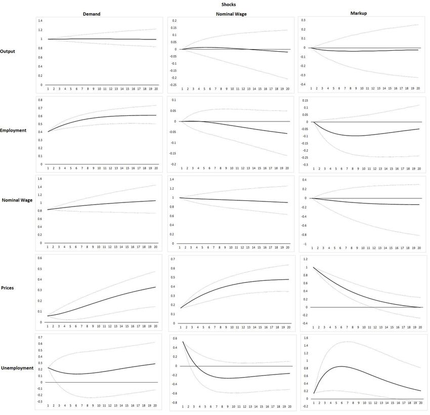
13Figure 6: Impulse Responses
A demand shock increases output, employment and nominal wages with persistent effects.
Although employment increases, there is no significant effects on unemployment. A tentative
explanation lies in the increase in nominal wage that acts as a shock absorber. A demand shock
expands the size of the labour force, and although employment rises, this does not necessarily
translate into a decrease in unemployment simply because the insiders benefit from higher
wages. This finding is even more peculiar when considering the response of the variables to a
wage shock. An increase in nominal wages does not have a significant impact on output and
14employment. However, it persistently increases prices while unemployment rises on impact.
Finally, a markup shock quasi permanently reduces employment and as a mirror effect, it raises
unemployment with a long lasting impact.
These findings are in line with prior expectations and have been long debated in the South
African literature. The structural nature of the unemployment is founded upon three main
pillars: nominal wages, prices and employment. An increase in wages due to the high bar-
gaining power of labour unions reduces the employable pool while keeping the insiders safe.
As a response, firms pass on this increase to the workers through a raise in prices given firms’
monopolistic structure in South Africa, inevitably translating into high and persistent unem-
ployment. This hysteresis effects is further emphasized by the considerable skill gap prevailing
in the labour market.
The forecast error variance decomposition (henceforth FEVD) consolidates these results.
This exercise investigates the contributions of all considered shocks in this scenario to a one-
step forecast error variance of each variables. We report the results in Figure 7 with a focus
on nominal wage, prices and unemployment.
Figure 7: Forecast Error Variance Decomposition
About 80 percent of nominal wage forecast error variance is explained by nominal wage
shocks. They remain important in the foreseeable horizon. The only additional and significant
contributor is the productivity shock but the impact is relatively low in comparison. This
finding emphasizes the rigid nature of wages which is consistent with the South African liter-
ature. The FEVD for prices displays a different story. Markup shocks explain for more than
90 percent of forecast error variance. However, this percentage reduces significantly as the
forecast horizon expands, with contributions from mainly nominal wage shock and productiv-
ity shock gaining in size. A similar observation is picked up for unemployment with markup
shocks contributing more to its forecast error variance as the horizon increases. This finding
15confirms the strong network between nominal wage, prices and unemployment explains for the
structural nature of the latter. The effects of an increase in nominal wage are transferred to
prices which ultimately results in persistently high unemployment.
3.3.2 Experimental scenarios
In this section we experiment with different versions of the baseline framework. First we control
for exogenous variables. Later on, these same variables will be endogenous to the framework
which has the advantage of assessing their impact on the baseline scenario. This is mainly
motivated by our wish to account for external shocks in our analysis and by the significance
of those shocks to the South African economy. Additionally, our choices are also influenced by
the robustness of these variables in estimating the historical decomposition of the core model1 .
We begin with the inclusion of the exchange rate as an exogenous. Fig 8 reports the impulse
responses to a devaluation shock.
1
The historical decomposition of the baseline framework is available in the Appendix
16Figure 8: Impulse Responses - Exogenous: Exchange Rate
This scenario has the advantage of improving the estimation of the output gap in the
historical decomposition2 . This is achieved while keeping the findings in the baseline scenario
fairly unchanged as shown in Fig 8 for the impulse responses and in Fig 9 for for the FEVD.
Noticeably however, nominal wage shocks grow in bigger proportion in explain forecast error
for prices while the effects of markup shocks in unemployment is relatively subdued compared
to the baseline as the forecast horizon increases.
2
See Appendix
17Figure 9: Forecast Error Variance Decomposition - Exogenous: Exchange Rate
We find similar results when using oil price and exchange rate as exogenous variables and
when we control for both oil price with the terms of trade. However, we couldn’t find any
conclusive results with the terms of trade as the single exogenous variable3 .
The next scenarios involve including the previously exogenous variables as endogenous to
the framework. The findings can be summarized as follows:
• Similar to the baseline scenario, adding more endogenous variables without controlling
for exogenous ones lead to a non-convincing estimation of the output gap in our opinion.
• Controlling for each exogenous variable or a combination of some in a six variables setup
yields different results. Regardless of the extra exogenous variables, some results are
robust. Therefore, a combination of oil price with terms of trade as exogenous to the
model has results similar to the baseline when we focus to the link between nominal
wages, prices and unemployment (i.e. nominal wage and markup shocks explain for the
hysteresis effect on unemployment). However, combining oil price with the exchange rate
subdues the long lasting effect of a markup shock on unemployment. It is important to
highlight that when convergence occurs, it does so after a considerable amount of time
has elapsed.
• The forecast error variance decomposition results remain robust throughout.
To illustrate the summarized findings, we report the case of the terms of trade added to
the baseline framework as an endogenous variable. Crude oil price (Federal Reserve Bank of
St Louis database) is used as an exogenous variable. We choose the terms of trade over the
3
All results are available upon request
18exchange rate based on two criterion: the marginal likelihood and the Deviance Information
Criterion (DIC). Figure 10 reports the impulse responses.
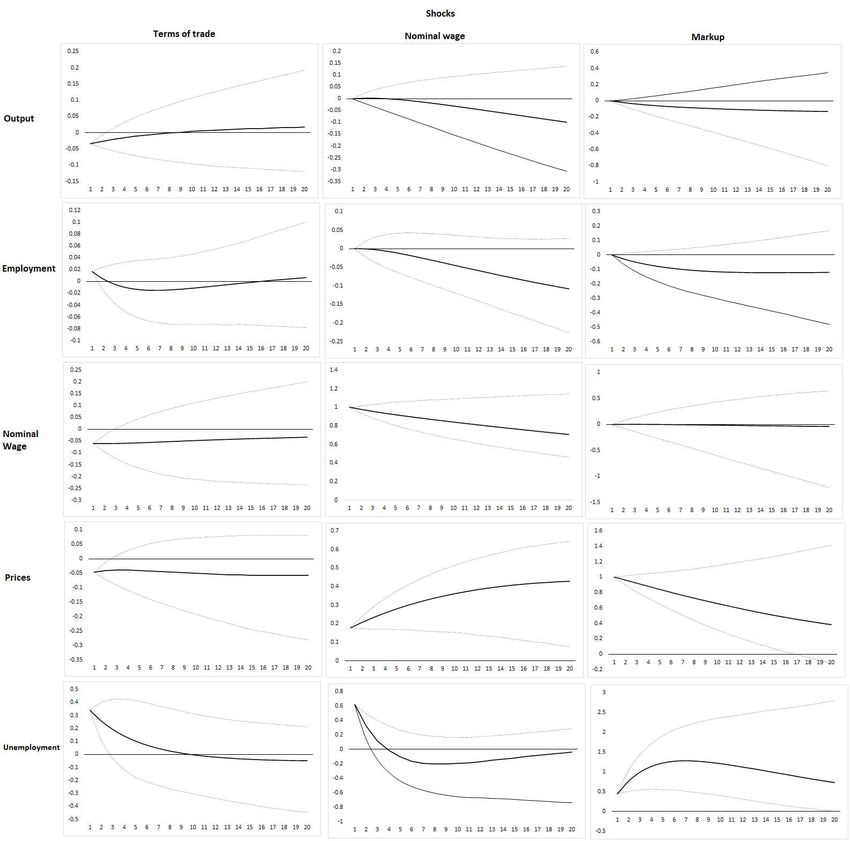
Figure 10: Impulse Responses - Baseline with Terms of Trade
A terms of trade shock does not very significantly impact the variables except for an increase
in unemployment that is however short lived. Nevertheless, the responses to nominal wage and
markup remain barely unchanged from the findings the baseline framework. This robustness is
confirmed with FEVD in Figure 11 with the only difference being the contribution of terms of
trade shocks in explaining unemployment. However, it is worth noticing that the contribution
19of terms of trade shocks in unemployment forecast error remain constant over the forecast
horizon.
Figure 11: Forecast Error Variance Decomposition - Baseline with Terms of Trade
It is therefore evident from this analysis that in the South African context there is a strong
connectivity between nominal wages, prices and unemployment. This is exacerbated by the
high bargaining power of workers combined with the significant skill gap in the labour mar-
ket that tend to favour skilled insiders when the economy emerges from a recession, therefore
keeping the unemployment consistently high. Considering the monopolistic structure of firms
in the economy makes matters worse because of their constant ability in transferring the cost
of increasing wages to workers through an increase in prices. The evidence of hysteresis in
unemployment shows the importance of reassessing the context in which policy in general is
conducted in South Africa, but particularly how forecast is dealt with. The forecast error vari-
ance decomposition shows consistent evidence of the importance of how the variables interact
with each. Ignoring the strong network between nominal wage, inflation and unemployment is
bound to yield bias forecast results which by ricochet will influence bias policy decision in the
context of an inflation targeting regime. In short, ignoring the importance of these variables
in the specification of the Phillips curve may yield flawed definition of the inflation target and
that of the output gap. Although the findings of this analysis gives us a different view on
the importance of understanding further the labour market and its complex interconnectiv-
ity with other prominent sectors in the functioning of the South African economy, it remains
evident that our knowledge of the labour market at a macroeconomic level remains limited.
Unemployment is a defining characteristic of the South African economy and as such, a further
investigation of the matter is required.
204 Conclusion
This paper investigates the presence of hysteresis in the South African labour market as an ex-
planation of the structural unemployment prevailing in the economy. The uses a simple model
of insider-outsider dynamics with hysteresis, which is later estimated using Bayesian VAR. The
model assumes full hysteresis, an assumption we could only make if the unemployment rate
series showed evidence of a unit root. We find it to be the case for South Africa. Additionally,
the baseline scenario shows that an increase nominal wage has permanent inflationary effects,
while a price markup shock induces a long lasting effect on unemployment. These results
associated with a relatively non responsive employment to shock indicate the main culprit in
explaining high persistent unemployment in South Africa. The findings are consolidated by the
forecast error variance decomposition in which nominal wages shocks contributes significantly
in explaining inflation forecast errors, and markup shocks become prominent contributors to
unemployment forecast errors as the horizon increases. This is robust when controlling for
additional exogenous and endogenous variables. Our results are in line with the literature that
explains persistence in unemployment after an adverse shock through the linkages between
nominal wages and prices. Specifically, workers benefiting from an increase in nominal wages
via the bargaining power of labour unions, bear the inflationary cost transfer to them by firms
operating in a monopolistic environment. This has important implications for the conduct of
monetary policy in South Africa. Particularly, a specification of the Phillips curve that ignore
the network link nominal wages and prices to unemployment is bound to yield flawed or simply
biased results.
21Appendix
Historical decomposition
Figure 12: Baseline
lny: Demand shock, lnn: Supply shock, lnnw: Nominal wage shock, lnp: Markup shock, lnulvl:
Labour shock. Any other colour represents variations in the data that exogenous and those
not explained by the model.
22Figure 13: Baseline with exogenous exchange rate
Figure 14: Baseline with endogenous terms of trade
lntot: Terms of trade shocks
23References
Blanchard, O. J. and D. Quah (1989). The dynamic effects of aggregate demand and supply
disturbances. The American Economic Review 79 (4), 655–673.
Blanchard, O. J. and L. H. Summers (1987). Hysteresis in unemployment. European Economic
Review 31 (1-2), 288–295.
Cross, R., M. Grinfeld, and H. Lamba (2009). Hysteresis and economics. IEEE Control Systems
Magazine 29 (1), 30–43.
Darby, J., A. H. Hallett, J. Ireland, and L. Piscitelli (1999). The impact of exchange rate
uncertainty on the level of investment. The Economic Journal 109 (454), 55–67.
Dolado, J. J. and J. F. Jimeno (1997). The causes of spanish unemployment: A structural var
approach. European Economic Review 41 (7), 1281–1307.
Galı́, J. (2015). Hysteresis and the european unemployment problem revisited. Technical
report, National Bureau of Economic Research.
Galı́, J. (2020). Insider-outsider labor markets, hysteresis and monetary policy. Technical
report, National Bureau of Economic Research.
Gambetti, L. and B. Pistoresi (2004). Policy matters. the long run effects of aggregate demand
and mark-up shocks on the italian unemployment rate. Empirical Economics 29 (2), 209–226.
Garga, V. and S. R. Singh (2021). Output hysteresis and optimal monetary policy. Journal of
Monetary Economics 117, 871–886.
Maidorn, S. (2003). The effects of shocks on the austrian unemployment rate–a structural var
approach. Empirical Economics 28 (2), 387–402.
O’Shaughnessy, T. (2011). Hysteresis in unemployment. Oxford Review of Economic Pol-
icy 27 (2), 312–337.
Piscitelli, L., R. Cross, M. Grinfeld, and H. Lamba (2000). A test for strong hysteresis.
Computational Economics 15 (1), 59–78.
24You can also read