Weakly-Supervised Classification and Detection of Bird Sounds in the Wild. A BirdCLEF 2021 Solution - arXiv

Weakly-Supervised Classification and Detection of
 Bird Sounds in the Wild. A BirdCLEF 2021 Solution
 Marcos V. Conde1,4 , Kumar Shubham2,4 , Prateek Agnihotri3,4 , Nitin D. Movva4 and
 Szilard Bessenyei
 1
 Universidad de Valladolid, Spain
 2
 Jio Saavn, India
 3
 Clairvoyant.ai, India
 4
 Equal contribution.

 Abstract
 It is easier to hear birds than see them, however, they still play an essential role in nature and they are
 excellent indicators of deteriorating environmental quality and pollution. Recent advances in Machine
arXiv:2107.04878v1 [cs.SD] 10 Jul 2021

 Learning and Convolutional Neural Networks allow us to detect and classify bird sounds, by doing this,
 we can assist researchers in monitoring the status and trends of bird populations and biodiversity in
 ecosystems. We propose a sound detection and classification pipeline for analyzing complex soundscape
 recordings and identify birdcalls in the background. Our pipeline learns from weak labels, classifies
 fine-grained bird vocalizations in the wild, and is robust against background sounds (e.g., airplanes, rain,
 etc). Our solution achieved 10th place of 816 teams at the BirdCLEF 2021 Challenge hosted on Kaggle.
 Code and models will be open-sourced at https://github.com/kumar-shubham-ml/kaggle-birdclef-2021.

 Keywords
 Audio Pattern Recognition, Audio Classification, BirdCLEF 2021, Birdcall identification, Computer Vision,
 Convolutional Neural Networks, Deep Learning, Sound Event Detection

 1. Introduction
 The BirdCLEF 2021 Challenge [1, 2] proposes to identify bird calls in soundscape recordings.
 The challenge was hosted on Kaggle from April 1, 2021 to June 1, 2021 1 .

 Dataset. The training set consists of short audio recordings of 397 bird species generously
 uploaded by users of xenocanto.org. These audio files have been downsampled to 32 kHz and
 converted to the format. In Section 3.1 we explain how we preprocess this short audios
 and generate curated audios and their corresponding Mel Spectrogram. The test set contains
 approximately 80 soundscape recordings in format (over 10 minutes of recordings), note
 that participants cannot access these audios. Additionally, recordings have associated metadata
 as the location (longitude, latitude), author, date, etc. Some of this features as the location can
 be especially useful for identifying migratory birds.

 CLEF 2021 – Conference and Labs of the Evaluation Forum, September 21–24, 2021, Bucharest, Romania
 " drmarcosv@protonmail.com (M. V. Conde); kumar.shubham@alumni.iitd.ac.in (K. Shubham)
 © 2021 Copyright for this paper by its authors. Use permitted under Creative Commons License Attribution 4.0 International (CC BY 4.0).
 CEUR
 Workshop
 Proceedings CEUR Workshop Proceedings (CEUR-WS.org)
 http://ceur-ws.org
 ISSN 1613-0073

 1
 https://www.kaggle.com/c/birdclef-2021/

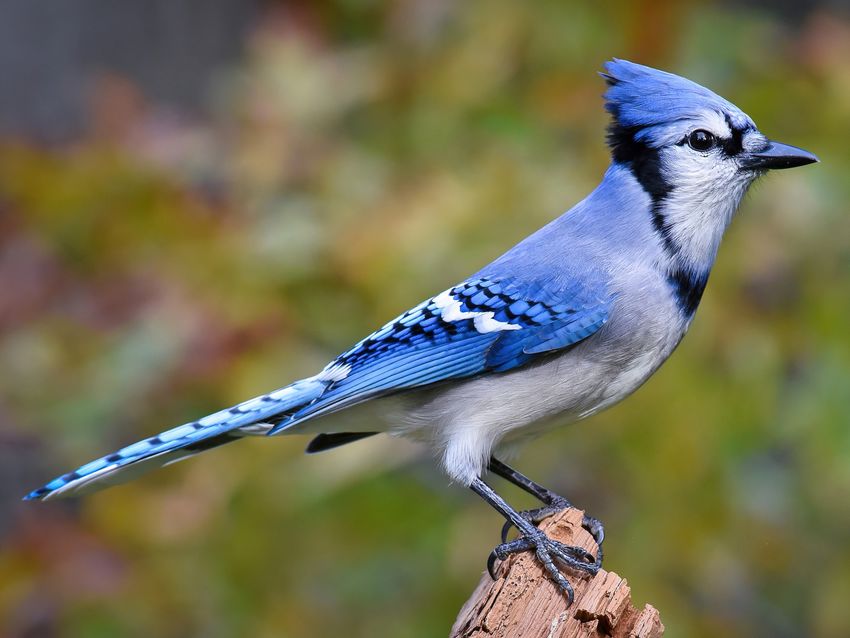
Problem. Given a long audio in format, participants have to predict if there is a bird
call in each 5-seconds segment of the given soundscape, and identify which of the 397 birds
is in such segment, thus, once the call is detected in a segment, the task can be considered as
fine-grained multi-label classification. Models infer on the test set with 3 hours run-time limit,
to ensure the efficiency of the solutions.

Evaluation. The performance is measured using the “micro averaged F1 score” and reported
on a Leaderboard (LB). Moreover, this leaderboard is divided into: “Public” which provides the
score on 28 test recordings (35%), and Private, which provides the score on 52 test recordings
(65%). During the competition, the participants only get feedback of their performance from the
public leaderboard, this is done to prevent overfitting.

 Train recordings were uploaded by the users of xenocanto.com from sites across the globe;
however, test recordings were from four places only:
 1. COL Jardín, Departamento de Antioquia, Colombia
 2. COR Alajuela, San Ramón, Costa Rica
 3. SNE Sierra Nevada, California, USA
 4. SSW Sapsucker Woods, Ithaca, New York, USA

 COL COR SNE SSW

Figure 1: Photographs of the four different sites from which audios were recorded.

 We define some terms related with this challenge that we will use in this work:
 • Leaderboard denoted as LB (including its two variants, public and private)
 • Cross-Validation denoted as CV.
 • the so-called ”score“ or ”metric“ refers to the official challenge metric: ”the row-wise
 micro averaged F1 score.“.
 • We refer to the ”Cornell Birdcall Identification - Kaggle 2020“ as the ”previous competition“,
 ”last year challenge“.
 • We define ”nocall“ as the class corresponding to the events in an audio where birdcalls are
 not detected. Other authors might also refer to this term as ”nosound“ or ”background“.
 This concept might be mentioned various times throughout the manuscript in different
 notations (“nocall”, nocall, no_call, etc).
 • Train soundscapes (or ”train soundscapes“) are 20 audio files that are quite comparable to
 the test set. They are all roughly ten minutes long and in the format.

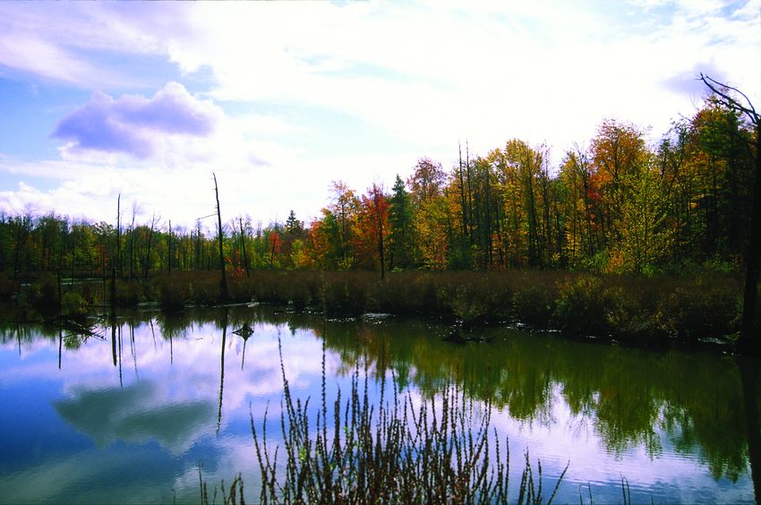
Blue 
  Jay 
  

Figure 2: Problem example. The audio in format can be visualized as a waveform (top) or a Mel
Spectrogram (bottom). We draw a red bounding box on the events in the audio where a birdcall is
detected, the other parts of the audio might contain background sounds or noise, such parts where
we do not detect a birdcall are also called ”nocall“ events. We detect the bircall in the audio, and also
identify the corresponding bird, in this case a ”Blue Jay“ (Cyanocitta cristata).

2. Related Work
Previous years BirdCLEF challenges proposed different problems related with large-scale bird
recognition in soundscapes or complex acoustic environments [1, 3, 4]. Sprengel et.al. [5]
and Lasseck [6, 7] introduced deep learning techniques for the ”Bird species identification in
soundscapes“ problem. State-of-the-art solutions are based on Deep Convolutional Neural
Networks (CNNs) [8, 9, 10], usually, deep CNNs with attention mechanisms are selected as
backbone in these experiments [11, 12, 13, 14, 15]. Pretrained audio neural networks (PANNs)
[14] provide a multi-task state-of-the-art baseline for audio related tasks, in previous competi-
tions these networks proved their generalization capability. Other approaches are focused on
Sound Event Detection (SED) [16, 17, 14, 18, 18], these approaches usually employ 2D CNNs to
extract useful features from the input audio signal (log-melspectrogram), these features still
contain information about frequency and time, then recurrent neural networks (RNNs) are used
to model longer temporal context from the extracted features or use directly the feature map to
predict, since it preserves time segment information.

3. Proposed Solution
In this Section we explain the main components of our solution to the BirdCLEF 2021 Birdcall
Identification Challenge. We base our solution on diverse and robust models trained on a
complete audio dataset using custom augmentations, and on a postprocess algorithm that
improves the predicted probabilities of bird appearances by using additional features as the site
(longitude, latitude), rarity of the bird, appearance of other birds in the audio, etc.

3.1. Dataset Preprocessing
We converted all the raw audio data to Mel Spectrograms using the library with each
having a length of 7 seconds and having some overlap 2 , we use this length instead of 5s
to ensure that the birdcalls are present in the clip. The Spectrograms were generated using
the following parameters: sample rate 32.000, 128 number of mels, minimum frequency 0
Hz, maximum frequency 16000 Hz, length of fast Fourier transform window (n-fft) 3200, and
number of samples between successive frames (hop-length) set to 80. We use the Cornell
Birdcall Identification 2020 Challenge dataset 3 as additional data, this dataset has 183 birds in
common and allowed us to add 1300 extra audio files. After some visual inspections of the Mel
Spectrograms, we determine a threshold such that the spectogram is considered to have weak a
signal or no signal, attending to its mean and maximum values. All the spectrograms with no
signal or very weak signals are removed and treated as noise. Once the above preprocessing
steps are completed, we split the training data into 5 different stratified folds.

3.2. Augmentations
We use 6 different types of augmentations in order to improve the robustness and generalization
capability of our models. In Figure 3 we show the effect of the proposed augmentations in
the same order we apply them: Mixing of images, Random Power, White noise, Pink Noise,
Bandpass noise, Lower the upper frequencies.
 First, 2 or 3 different training images are overlapped on each other with a random probability
of mixing (default is 0.7). Once this is completed random power is applied on the mixed image
to bring all the images to a certain contrast and brightness level. Next we add augmentations in
the following order: white noise, pink noise, bandpass noise, reducing upper level frequencies,
we found experimentally that this is the optimal order. All the augmentations mentioned above
are added with a probability between 0.4 and 0.7 to ensure the diversity of the data.

Figure 3: Visualization of our augmentation pipeline explained in Section 3.2.

 2
 https://www.kaggle.com/kneroma/kkiller-birdclef-2021
 3
 https://www.kaggle.com/c/birdsong-recognition

3.3. Models
In Table 1 we show the model architectures used in our experiments. All the models had similar
performance on out-of-fold validation using 5 stratified folds. Single models perform reasonably
good, but combining them into an ensemble provided best performance as we explain in Sections
3.5 and 4. In our experiments we found that bigger architectures did not necessarily provide
better results. Hence, a lot of experimentation was done with smaller models such as ResNeSt-50
[11] and EfficientNet-B0 [12]. In addition to the proposed models, we use top models from the
Cornell Birdcall Identification 2020 Challenge 4 , in Section 4 we explain how we incorporate
the following models into our ensemble:
 1. The 1st place solution there are 14 models in total, all of which are PANN DenseNet-121
 architecture with an added attention layer. The models were trained with 264 classes of
 bird data and augmentations such as SpecAugmentation, gaussian noise, gain (volume
 adjustment), along with mixup for some models were used to increase model’s robustness.
 2. The 2nd place solution. Two different models: ResNet-50 and EfficientNet-B0. Both these
 architectures were trained with different settings on 264 birds and were trained directly
 on mel spectrograms instead of training on the audio files.

Figure 4: Example of multilabel classification model pipeline. During training, the generated Mel
Spectrogram (see Section 3.1) is augmented as explained in Section 3.2. In this diagram we do not show
additional postprocess of the predictions.

3.4. Training Details
We use a GPU RTX-2070 with 8 GB VRAM for training our models, training time for each model
on this device is reported on Table 1. In all the experiments we train for 60 epochs, we use batch
size 64 and Adam Optimizer [19]. We use a Binary Cross Entropy loss function implemented as
in PyTorch with Label Smoothing [20]. Additionally we use a Learning Rate Scheduler based on
Cosine Annealing with base LR of 0.001 [21]. During training we track the loss function, F1
score, Precision, Recall, Label ranking average precision score for both training and validation
data. See Figure 5 as an example of our training metrics monitoring.

3.5. Inference and Postprocessing
We use the provided ”train soundscapes“ audio samples as validation set. These audios were
much noisier than the curated ones used for training (see Section 3.1) and closely resemble ”test
 4
 https://www.kaggle.com/c/birdsong-recognition

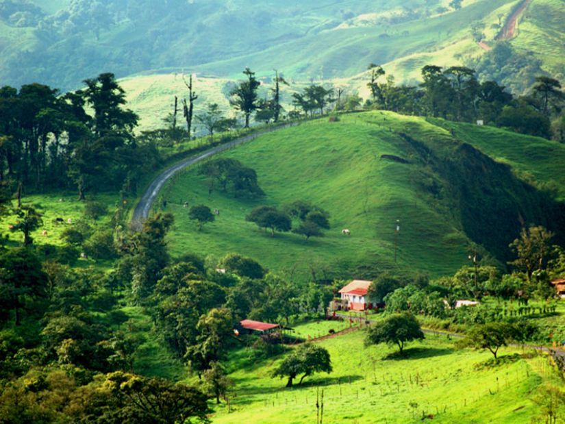
Figure 5: Loss and validation metrics evolution during training of ResNeSt-50 model. Note that the
training loss is higher than the validation loss because augmentations were only applied during training.

Table 1
Ablation study of our models trained from scratch on the BirdCLEF 2021 dataset. The training time
depends on the number of augmentations, architecture and batch size. The corresponding Out-Of-Fold
(5-fold) F1 score for each model and the validation score using Train Soundscapes (TS) are provided.
Models with ResNeSt as backbone have better performance than DenseNet or EfficientNet.
 Architecture OOF F1 Score TS F1 Score No. Parameters Time (min) × Epoch
 ResNeSt-50 [11] 0.755 0.706 26,247.693 20
 ResNeSt-101 [11] 0.748 0.705 47,039.469 34
 ResNeXt-50_32x4d [13] 0.714 0.63 23,793.357 22
 SeResNet-50 [22] 0.725 0.674 26,852.477 25
 DenseNet-121 [23] 0.718 0.66 7,360.781 17
 EfficientNet-B0 [12] 0.722 0.691 4,516.105 15

soundscapes“. The distribution of birds in these soundscapes was also different from the training
short audios. However, there were only 20 soundscape clips, which covered only 48 of 397 bird
classes and 2 of 4 possible sites, making it too challenging to train acoustic models on these
clips. The training short audios were only labelled at clip level, but the long audio predictions
were generated at frame level (frame of 5 seconds). The noisy labels led to a significant gap
between the performance of our models on short audios (reported at Table 1) and this validation
set. For these reasons, the ”train soundscapes“ clips were used only for validation purposes and
to achieve better generalization.
 A series of post-processing strategies were employed to bridge the gap between performance
on short, cleaner audio and soundscapes. Our post-processing improved the cross-validation
(CV) and Leaderboard F1 score (LB) by 0.008-0.01.
 Initially, we infer all 5-second clips at a stride of 1 second. Our final submission consists of
an ensemble of 13 different models explained at Section 3.3. The ensemble optimized weights
were calculted based on the validation set. A second-stage model, Support Vector Classifier, was
trained with a leave-one-clip-out validation strategy on the 20 train soundscapes. This model

computes calibrated confidence based on some frame-based, clip-based, and distance-based
features generated from probabilities per inference step, in addition to latitude and longitude
information for the sites. During the training of the second-stage model, bird information
was masked to help the model generalize well on birds absent in train soundscapes. Finally,
we further improve our performance by using a series of False-Positives and False-Negatives
reduction techniques and the use of two different thresholds for bird call or ”nocall“ identification
and bird categorization. We reduced the false negatives by increasing the confidence of most
frequent birds from each site by 0.1. This strategy worked well both on CV and public/private
LB. Therefore, there were three types of predictions, (a) only birds, (b) only nocall (no birds),
and (c) both nocall and birds.

3.5.1. Second-Stage Model
The CNN model we trained had some limitations. The short train audio was labelled only at the
clip level. On analysing train soundscapes, we found that if a bird is found anywhere in the
clip, it increases the chances of finding the same bird at other places in the clip. Furthermore,
the chances of finding the birds in immediate neighbour frames would also be high. This phe-
nomenon encouraged us to train a second stage model on train soundscapes which calibrates
the confidence using some frame-based and clip-based features. Some of the challenges in
training the second stage model involved the limited number of birds and sites in train sound-
scapes, which could hurt the model’s generalisation capability. To solve this, we converted the
multi-label problem into a binary classification problem and masked the information about
birds for this second stage model. We started with training a simple logistic regression model
where each unique tuple of (clip, 5-second frame, bird) constitutes a single training sample. No
information about bird class was passed in any way directly to the model. This post-processing
alone gave a 0.005-0.007 boost on CV and public/private LB. We saw further improvement
(+0.002) by adding location-based features and switching from logistic regression to support
vector machines. Only four features were used for training the second-stage model. For example,
let us denote the probability generated for a 5-second frame ending at seconds for any bird
B in the clip by . Let the length of the clip be seconds ( = 600 for all soundscapes).
The calculation details of these features for the frame ending at seconds for the bird B are
explained below:
 1. Frame-based features: Rolling Mean 3 ( 3 ) and Rolling Mean 9 ( 9 )
 +1
 1 ∑︁
 3 = 
 3
 = −1
 +4
 1 ∑︁
 9 = 
 9
 = −4
 2. Clip-based features:

 = ( 5 , . . . , )
 3. Distance-based features (minimum Haversine distance) explained in Section 3.5.2.

3.5.2. Minimum Haversine Distance
The haversine distance [24] is an excellent approximation for the angular distance between
two points expressed as latitudes and longitudes on earth. The minimum haversine distance
is expressed as the distance between a site and a bird class. Let us suppose that a bird class
has 400 samples in the train short audios. First, the haversine distance is calculated between
the position of each of those birds and the site’s location. The minimum of the set of these 400
distances is called minimum haversine distance.

3.5.3. False Positives Reduction
All the (bird, site) pairs satisfying at least one of the following conditions were discarded:
 1. Minimum Haversine Distance between site and bird is greater than 100. Analysing train
 soundscapes, we found that only 3 (birds, site) pairs found in train soundscapes have a
 minimum haversine distance greater than 60. So, all the (birds,site) pairs with minimum
 haversine distance>100 were rejected.
 2. Probabilities generated directly from the ensemble for that frame were less than 0.01. This
 post processing helped us get small boost in CV and private LB and helped us reduced
 training data for Support Vector Classifier.
 3. Remove birds belonging to one of the following classes - (Great Horned Owl, Plumbeous
 Pigeon). As we analysed the train soundscapes, we found that our models have a very high
 False Positives Rate for these species. Most of the time, when the model was predicting
 these classes, the actual target was nocall.

3.5.4. Confidence Thresholds
Two sets of thresholds were used for calibrating confidence. The nocall confidence was deter-
mined as 1 − (calibrated confidence for all birds for that 5-second frame). The first thresh-
old was applied on nocall confidence (no birds detected). All 5-second frames having nocall
confidence above this threshold contained nocall as one of the predictions. The second threshold
was applied on calibrated confidence for each bird.

4. Experimental Results
4.1. Evaluation of Methods
We trained models using short train audios as explained in Section 3.1. We use long soundscape
audios for training probability calibration (PC) model, for optimizing false-negative reduction
(FNR) and false-positive reduction (FPR) methods, tuning thresholds, and for computing the
validation scores (see Section 3.5). For model selection, we kept track of both call and nocall
F1 scores to make sure that models are not heavily affected distribution of nocall-call samples.
Note that Train soundscapes had around 63% nocall samples, and we estimate that the hidden
test fraction corresponding to the public LB has 54% nocall samples. We rely on two different
validation scores: the ”High nocall Validation Score“ denoted as HNVS and the ”Low nocall
Validation Score“ denoted as LNVS. In Equation 1 we show the definition of both metrics:

HNVS (CV@0.63) = 0.63 × F1-micronocall + 0.37 × F1-microcall
 (1)
 LNVS (CV@0.54) = 0.54 × F1-micronocall + 0.46 × F1-microcall
 In order to make sure that our models generalizes to unseen data (e.g. private LB), we
separately calculated row-wise micro averaged F1-score for samples having bird calls and
samples having no bird call. Table 2 shows the different metrics that we considered for selecting
our models and experiments and the ablation study of the different postprocess steps. For further
validation, we also tested our models on the Cornell Birdcall Identification 2020 Challenge
leaderboard 5 . Last year competition data had 3 different sites,after some analysis, we found
that site2 was close to SSW site and site1 was close to SNE site. Also we estimated that this test
data has around 57% nocall samples.

4.2. Results and Comparison
Table 2 summarizes our experiments. We bagged 13 CNN-based models (Section 3.3) with
CV@0.63 (HNVS) varying from 0.68 to 0.71. These 13 models were different in terms of
augmentation strategy and architecture. Adding augmentations improved the true positive rate
of these models and reduced the difference of scores between the predictions on short audios
and train soundscapes(relatively noisier), thus making models robust against the anthropogenic
noise. The bagging of these 13 models gave 0.74 CV@0.54 for COR site but was not that effective
on SSW sites. For SNE & SSW sites, we fine-tuned the last year competition first and second
place models (only for birds having minimum Haversine distance lesser than 100 for these two
sites). Using these models improved the CV@0.54 for SNE & SSW sites from 0.69 to 0.75.

Table 2
Row-wise micro averaged F1-score results of models on Public-Private LB, and ”train soundscape“
validation. For local validation, row-wise micro averaged F1-score was calculated on samples with call
and no_call separately, and the metric CV@0.54 (LNVS) was also calculated.
 Method All Sites (2021) COR Site SSW Site COR & SSW Sites
 Public LB Private LB No call Call CV@0.54 No call Call CV@0.54 No call Call CV@0.54
 SNE & SSW site models - - - - - 0.9094 0.5552 0.7465 - - -
 All site models 0.7155 0.6203 0.9300 0.5208 0.7418 0.9431 0.3876 0.6875 0.9261 0.4623 0.7127
 Ensemble 0.7499 0.6450 0.9300 0.5208 0.7418 0.8923 0.5861 0.7514 0.9130 0.5591 0.7502
 Ensemble + PC 0.7744 0.6609 0.9187 0.6415 0.7912 0.8869 0.6106 0.7598 0.9044 0.6234 0.7751
 Ensemble + PC + Site-info 0.7711 0.6722 0.9106 0.6756 0.8025 0.8725 0.6327 0.7622 0.8934 0.6505 0.7816
 Ensemble + PC + FNR 0.7774 0.6630 0.9086 0.6758 0.8015 0.8720 0.6354 0.7632 0.8921 0.6521 0.7817
 Ensemble + PC + FNR + FPR 0.7754 0.6780 0.9285 0.6583 0.8029 0.8836 0.6343 0.7656 0.9082 0.6443 0.7836
 Selected Submission 0.7801 0.6738 0.9106 0.6756 0.8025 0.8754 0.6363 0.7654 0.8947 0.6526 0.7834

 As shown in Table 2, the time series-based probability calibration (PC) model provided a
good improvement in CV and LB. Using the clip-level and the neighboring frames information,
the probability calibration model improved CV on samples having bird call by +0.07, and raised
Public LB to 0.774 and Private LB to 0.661. Then the bird-to-site mapping (site-info) using
minimum Haversine distance helped in two ways: (i) reducing false-negatives by reducing the
call identification thresholds of the most frequent birds, (ii) reducing false positives by removing
the birds in the predictions which are not found at a particular site.
 5
 https://www.kaggle.com/c/birdsong-recognition/leaderboard

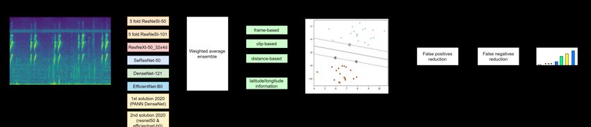
Figure 6: Overview of our solution pipeline. We show an ensemble of various models, our SVC model for
probability calibration (PC) and the proposed probability filters for False-Positives and False-Negatives
reduction.

Table 3
Comparison of our solution ot the BirdCLEF 2021 Challenge (see Section 3) and the winning solutions
of the Cornell Birdcall Identification 2020 competition on its Leaderboard (public and private). Our
solution generalizes to different sites and extends previous approaches improving performance.
 Model Cornell Birdcall Identification 2020
 Public LB Private LB
 Ours (BirdCLEF 2021) 0.659 0.699
 Birdcall 2020 - 1st place 0.624 0.681
 Birdcall 2020 - 2nd place 0.628 0.677
 Birdcall 2020 - 3rd place 0.626 0.675

Further reducing false negatives via removing birds from the predictions which are most
commonly confused with ”nocall“ helped in achieving CV@0.54=0.7836 and Private LB=0.6780.
Additionally, we compare our current solution against previous state-of-the-art methods for
this challenge by submitting our solution to Cornell Birdcall Identification 2020 Challenge. Our
solution was able to give significantly better results than previous winning solutions of the
Cornell Birdcall Identification 2020 Challenge (see Table 3). There is a gain of +0.035 on Public
LB and a gain of +0.018 on Private LB as compared to 2020 first place solution. We understand
that our model is an extension of previous state of the art, and can generalize to detect all variety
of birds from unknown sites and background sounds.

5. Conclusion and Future work
We aim to help researchers monitoring birds and automatically intuit factors about an area’s
quality of life, levels of pollution, and the effectiveness of restoration efforts. We present a
sound detection and classification pipeline for analyzing soundscape recordings that learns from
weak labels, classifies fine-grained bird vocalizations and is robust against anthropogenic or
natural noisy sounds (e.g., rain, cars, etc). Our solution achieved 10th place of 816 teams at the
BirdCLEF 2021 Challenge. We would like to improve efficiency and usability, and thus, use this
pipeline online or on smartphones. To achieve this, we are exploring Knowledge Distillation to
reduce notably the hardware requirements and inference time.

Acknowledgments
We would like to thank Kaggle and Dr. Stefan Kahl for hosting the BirdCLEF 2021 Challenge.
We also want to thank participants of the Cornell Birdcall Identification 2020 Challenge and
this challenge for sharing insights, datasets, their solutions and open-sourced code, especially:
Ryan Wong, Kramarenko Vladislav, Hidehisa Arai, Kossi Neroma, Jean-François Puget (CPMP).

References
 [1] S. Kahl, T. Denton, H. Klinck, H. Glotin, H. Goëau, W.-P. Vellinga, R. Planqué, A. Joly,
 Overview of BirdCLEF 2021: Bird call identification in soundscape recordings, in: Working
 Notes of CLEF 2021 - Conference and Labs of the Evaluation Forum, 2021.
 [2] A. Joly, H. Goëau, S. Kahl, L. Picek, T. Lorieul, E. Cole, B. Deneu, M. Servajean, R. Ruiz De
 Castañeda, I. Bolon, H. Glotin, R. Planqué, W.-P. Vellinga, A. Dorso, H. Klinck, T. Denton,
 I. Eggel, P. Bonnet, H. Müller, Overview of LifeCLEF 2021: a System-oriented Evaluation
 of Automated Species Identification and Species Distribution Prediction, in: Proceedings
 of the Twelfth International Conference of the CLEF Association (CLEF 2021), 2021.
 [3] S. Kahl, M. Clapp, W. Hopping, H. Goëau, H. Glotin, R. Planqué, W.-P. Vellinga, A. Joly,
 Overview of BirdCLEF 2020: Bird Sound Recognition in Complex Acoustic Environments,
 2020.
 [4] S. Kahl, F.-R. Stöter, H. Goëau, H. Glotin, B. Planqué, W. Vellinga, A. Joly, Overview of
 BirdCLEF 2019: Large-Scale Bird Recognition in Soundscapes, in: CLEF, 2019.
 [5] E. Sprengel, M. Jaggi, Y. Kilcher, T. Hofmann, Audio based bird species identification using
 deep learning techniques, in: CLEF, 2016.
 [6] M. Lasseck, Bird species identification in soundscapes, in: CLEF, 2019.
 [7] M. Lasseck, Audio-based bird species identification with deep convolutional neural net-
 works, in: CLEF, 2018.
 [8] J. Schlüter, Bird identification from timestamped, geotagged audio recordings, in: CLEF,
 2018.
 [9] J. Bai, C. Chen, J. Chen, Xception based method for bird sound recognition of birdclef 2020,
 in: CLEF, 2020.
[10] M. Mühling, J. Franz, N. Korfhage, B. Freisleben, Bird species recognition via neural
 architecture search, in: CLEF, 2020.
[11] H. Zhang, C. Wu, Z. Zhang, Y. Zhu, H. Lin, Z. Zhang, Y. Sun, T. He, J. Mueller, R. Manmatha,
 M. Li, A. Smola, Resnest: Split-attention networks, 2020. arXiv:2004.08955.
[12] M. Tan, Q. V. Le, Efficientnet: Rethinking model scaling for convolutional neural networks,
 2020. arXiv:1905.11946.
[13] S. Xie, R. Girshick, P. Dollár, Z. Tu, K. He, Aggregated residual transformations for deep
 neural networks, 2017. arXiv:1611.05431.
[14] Q. Kong, Y. Cao, T. Iqbal, Y. Wang, W. Wang, M. D. Plumbley, Panns: Large-scale pretrained
 audio neural networks for audio pattern recognition, 2020. arXiv:1912.10211.
[15] K. He, X. Zhang, S. Ren, J. Sun, Deep residual learning for image recognition, 2015.
 arXiv:1512.03385.

[16] K. Drossos, S. Mimilakis, S. Gharib, Y. Li, T. Virtanen, Sound event detection with depthwise
 separable and dilated convolutions, 2020, pp. 1–7. doi:10.1109/IJCNN48605.2020.
 9207532.
[17] E. Fonseca, M. Plakal, D. P. W. Ellis, F. Font, X. Favory, X. Serra, Learning sound event
 classifiers from web audio with noisy labels, 2019. arXiv:1901.01189.
[18] V. Lostanlen, J. Salamon, A. Farnsworth, S. Kelling, J. Bello, Robust sound event detection
 in bioacoustic sensor networks, PLOS ONE 14 (2019) e0214168. doi:10.1371/journal.
 pone.0214168.
[19] D. P. Kingma, J. Ba, Adam: A method for stochastic optimization, 2017. arXiv:1412.6980.
[20] R. Müller, S. Kornblith, G. Hinton, When does label smoothing help?, 2020.
 arXiv:1906.02629.
[21] I. Loshchilov, F. Hutter, Sgdr: Stochastic gradient descent with warm restarts, 2017.
 arXiv:1608.03983.
[22] J. Hu, L. Shen, S. Albanie, G. Sun, E. Wu, Squeeze-and-excitation networks, 2019.
 arXiv:1709.01507.
[23] G. Huang, Z. Liu, L. van der Maaten, K. Q. Weinberger, Densely connected convolutional
 networks, 2018. arXiv:1608.06993.
[24] H. Mahmoud, N. Akkari, Shortest path calculation: A comparative study for location-based
 recommender system, in: 2016 World Symposium on Computer Applications Research
 (WSCAR), 2016, pp. 1–5. doi:10.1109/WSCAR.2016.16.