The Master-Curve Band considering Measurement and Modeling Uncertainty for Bituminous Materials

Hindawi
Advances in Materials Science and Engineering
Volume 2021, Article ID 5543279, 11 pages
https://doi.org/10.1155/2021/5543279

Research Article
The Master-Curve Band considering Measurement and Modeling
Uncertainty for Bituminous Materials

 Quan Liu ,1 Jiantao Wu ,2 Pengfei Zhou ,2 and Markus Oeser 1

 1
 Institute of Highway Engineering, RWTH Aachen University, Aachen 52074, Germany
 2
 College of Civil and Transportation Engineering, Hohai University, Nanjing 210037, China

 Correspondence should be addressed to Jiantao Wu; jiantao.wu@hhu.edu.cn

 Received 24 January 2021; Revised 13 February 2021; Accepted 19 February 2021; Published 25 February 2021

 Academic Editor: Shuaicheng Guo

 Copyright © 2021 Quan Liu et al. This is an open access article distributed under the Creative Commons Attribution
 License, which permits unrestricted use, distribution, and reproduction in any medium, provided the original work is
 properly cited.
 This paper proposes using the master-curve band (MCB) to incorporate the unavoidable measurement errors and modeling
 uncertainty into the bitumen master-curve construction. In general, the rheological property of bitumen within the linear
 viscoelastic region is characterized by the master curve of modulus and/or phase angle, provided that the bitumen complies with
 the time-temperature superposition principle (TTSP). However, the master-curve construction is essentially a mathematical
 fitting process regardless of whether or not the original data is perfect enough to fit. For this reason, the MCB was introduced to
 consider the uncertainty information instead of a single master curve. Rheological data of four kinds of bitumen including unaged
 and aged bitumen were used to construct the MCBs. The results indicated that the generalized sigmoidal model showed the widest
 master-curve band, followed by Christensen-Anderson-Marasteanu (CAM) and CAM (Gg ) models. The width of MCB was a
 useful tool to identify the sensitivity of bitumen to rheological models. The sensitivity of bitumen to rheological models is
 associated with the number of active parameters in rheological models and model parameters’ confidence intervals. The
 construction of an MCB was beneficial to select the rheological models. Accordingly, the CAM (Gg ) model is proved to be the best
 to analyze the aging effects.

1. Introduction It is worth noting that the complex shear modulus and
 phase angle of bitumen only make sense with a given tem-
Most of the distresses that occur in asphaltic pavements are perature and loading frequency. However, the property of
associated with the binder phase in asphalt mixtures, such as bitumen under a single condition of temperature and loading
adhesion failure (moisture damage) [1, 2], cohesion failure frequency is not sufficient to reveal the entire performance of
within bitumen (cracking) [3], fatigue failure [4, 5], and bitumen in a broad range of temperature and frequency. For
permanent deformation (rutting) [6]. In the characterization this reason, Airey [8] proposed the black diagram to identify
of bitumen’s physical properties, rheological behavior was the rheological performance without considering the tem-
stressed due to its close connection to the above distresses perature and frequency. To date, the black diagram has been
[7]. The terminology rheology was conceptualized as the successfully used in many studies of bitumen rheology
study of deformation and flow properties of materials [8]. [7, 10, 11]. However, the black diagram is not able to reveal the
Bituminous material is manifested as being viscoelastic, temperature or frequency sensitivity of bitumen. Alternatively,
showing typical time- and temperature-dependent proper- the master curve of modulus or phase angle was proposed to
ties [9]. By far, the rheological properties of bitumen are handle the rheological data [12–14]. The master-curve con-
conventionally represented by two primary parameters, struction introduced a time-temperature shift factor to bring
which are complex shear modulus (G∗) and phase angle (δ) rheological data measured at different temperatures and fre-
measured through the dynamic shear rheometer (DSR). quencies to one overall continuous curve. The preparatory

2 Advances in Materials Science and Engineering

work required for constructing the master curve is to deter- variation of shift factors usually depends on the rheological
mine the shift factor as a temperature function. Many ap- model selection. In this case, unavoidable uncertainty
proaches were proposed to determine the temperature mainly rests on the measurement error, model variation, and
dependence of shift factors [15], such as a manual procedure fitting variation.
[16], the Arrhenius equation [17], the Williams-Landel-Ferry Based on the above analysis, finding an approach that
(WLF) formula [18], logarithmic-linear relationship with incorporates uncertainty information into the master curve
temperature [19], the Fox method [20], and viscosity-tem- could benefit a more accurate estimation of bitumen rhe-
perature susceptibility (VTS) method [21]. ological properties. For this reason, this study proposed a
 In addition to the determination of shift factors, rhe- method to consider the uncertainty that exists in master-
ological models are usually used to achieve a perfectly curve construction by extending a master curve to a master-
smooth master curve. Yusoff et al. [22] classified rheo- curve band (MCB). The MCB has the following potential
logical models into three categories: nonlinear multivari- advantages compared with the master curve: (1) the un-
able models, empirical algebraic equations, and mechanical certainty information is included in the master-curve band;
element models. The nonlinear multivariable models are (2) the sensitivity of bitumen to the rheological model can be
not usually used as they are empirical models presented in quantitatively featured; and (3) the MCB can help select
the form of a figure. The empirical algebraic equations, such appropriate rheological models to study the aging or
as the sigmoidal model and Christensen-Anderson-Mar- modification effect.
asteanu (CAM) model, and mechanical element models,
such as the 2S2P1D model, were extensively adopted in 2. The Development of the Master-Curve Band
many kinds of research. The measured rheological data is
mathematically fitted through an optimization process, 2.1. Data Variation Measured by DSR. In the first phase of
converting into the master curve at the reference tem- the RILEM Round Robin Binder Fatigue Test mentioned
perature. Herein, it is noticeable that the achieved mater above, it was found that the coefficient of variation (COV)
curve, to some extent, mathematically approximates the measured for complex modulus was 15.6%, and, for phase
experimental data. However, uncertainty in the above angle, the maximum coefficient of variation observed was
process could cause significant variation between experi- 3.7% [25]. After improving the test protocols, in the second
mental and predicted data. Figure 1 illustrates the potential phase of their study, the variation coefficient changed to
uncertainty factors that could give rise to variation between 6.7% and 4.8% for complex modulus and phase angle, re-
measurement and prediction. spectively [25]. Although this study was carried out to
 Among these potential uncertainty factors shown in identify reasonable fatigue test methods, the results indi-
Figure 1, sample variation can be eliminated by measuring cated that DSR measurement showed unavoidable mea-
multiple parallel samples. As for the testing protocols, some surement errors for complex modulus and phase angle.
efforts have been made toward accurate measurement for Besides, the measurement error of the complex modulus is
decades. Carswell et al. [23] discussed testing protocols that much more significant than that of the phase angle. Un-
might cause measurement variation: temperature control, fortunately, a single master-curve cannot include the data
sample geometry, sample preparation, equipment calibra- variation in its current presentation form.
tion, linear range, and so forth. In their discussion, tem-
perature control and sample geometry are two critical
 2.2. Model Variation Caused by Model Types and Fitting
sources of errors. With the development of the device and
 Process. Many linear viscoelastic rheological models have
correlation method, temperature control is no longer an
 been developed to construct the master curve of bitumen.
issue if the standard procedure is followed. The geometry
 Empirical equations such as CAM and mechanical models
size effect can be eliminated by using appropriate testing
 such as the 2S2P1D model have been successfully applied to
plates [8]. The bitumen sample showed high modulus in
 characterize the bitumen viscoelastic properties. Nur et al.
some conditions, and the compliance error could induce
 compared several mathematical models applied to the
inaccurate measurement. Correspondingly, Wu et al. [24]
 unaged, aged, and modified bitumen binders [26]. The re-
proposed an efficient method to correct rheological data’s
 sults showed that the generalized sigmoidal model per-
compliance error using the 2S2P1D model.
 formed the best in terms of the goodness of fit, while the
 Nonetheless, the measurement uncertainty caused by
 CAM model was reported to be senior to other models.
laboratory or technician difference cannot be avoided (re-
 Nonetheless, modeling sensitivity has not been thoroughly
ferring to measurement error in Figure 1). A study launched
 investigated. One rheological model might be powerful
by RILEM investigated the repeatability of binder fatigue
 enough to satisfy measurement data. However, it cannot
tests [25]. This study invited varying laboratories to measure
 exclude the possibility of overfitting. Therefore, a good
the same type of bituminous materials. In this report, the
 quality model should show the goodness of fit and efficiently
coefficient of variation measured for complex modulus was
 identify the variation caused by data variation and modeling
up to 15.6%. It is illustrated that the measurement error of
 uncertainty.
rheological properties is practically unavoidable.
 On the other hand, in the practical realization of the
master curve, the determination of shift factors is flexible 2.3. Quantitative Description of Data Variation and Modeling
toward a goodness of fit of rheological models. Therefore, the Uncertainty. This section introduced how to consider the

Advances in Materials Science and Engineering 3

 Sensitivity
 Sample variation
 Factor 1

 Sample preparation and data collection
 Testing protocols

 Model selection
 Factor 2
 Measurement errors

 Variation of shift
 factors

 Model variation Factor 3

 Fitting variation

 Characterization & Potential
 Uncertainty evaluation
 sample testing uncertainty factors

 Figure 1: Qualitative analysis of uncertainty factors in master-curve construction.

data variation and modeling uncertainty quantitatively. As The generalized sigmoidal model was proposed to de-
previously noted, the unavoidable data variation could reach scribe the stiffness of asphalt mixtures. It has been proven
up to 15.6%. Therefore, the measured data was extended by applicable to the bituminous binder and other materials, as
multiple corresponding coefficients of variation, as shown in shown in the following equation [28]:
Figure 2(a). Seven data groups, including the measured one, α
were calculated. log G∗ � δ + 1/λ
 ,
 (2)
 1 + λe {
 (β+c log(2πf)})
 Seven data groups were then subjected to the con- 
struction of a master curve using a specific rheological
model. In this case, seven groups of model parameters can be where G∗ is the complex modulus and f is the reduced
obtained. It is time-consuming to conclude the distribution frequency. δ, α, β, λ, and c are model parameters.
of model parameters experimentally. Alternatively, in pre- According to the time-temperature superposition
vious literature, it was reported that measurements of as- principle, the complex modulus measured at temperature T
phalt mixtures reasonably approximate a normal and frequency f can be obtained at reference temperature
distribution curve [27]. Therefore, it was assumed that the Tref. The reduced frequency is determined through the shift
distribution of model parameters caused by modeling un- factor, as expressed in the following equation [29]:
certainty also complies with the normal distribution, as
 G∗ T, αT · f � G∗ Tref , f . (3)
shown in Figure 2(b).
 Moreover, this study considered three confidence levels The construction of the master curve was performed
(95%, 90%, and 85%) to study the model sensitivity of bi- with the aid of the Solver function in Excel. Combining
tumen. It should be stressed that this study only focuses on equation 1 with equation 3, the master curve can be derived
the development of a master-curve band for complex by optimizing the parameters with nonlinear least-square
modulus. However, the master-curve band’s construction regression methods. In particular, this method minimized
for phase angle can also be achieved following the identical the sum of square errors (SSE) between measured data and
procedure proposed in this study. predicted data, which can be written as follows [30]:
 2
 ​ log|G∗ (f, T)| − log G∗ 
 mea mod αT T, Tref · f, Tref 
2.4. The Mathematical Expression of a Master-Curve Band. SSE � ∗ 2 .
 log Gmea (f, T) 
For example, the rheological model, namely, the generalized
sigmoidal model and the Williams-Landel-Ferry (WLF) (4)
formula, was used to construct the master curve. The WLF
equation is as follows [15]: The model parameters were achieved by solving equation
 4, consisting of a parameter vector x � (x1, x2, · · ·, xn). It is
 − C1 T − Tref hypothesized that individual parameters are independent of
 log αT � , (1)
 C2 + T − Tref each other. As introduced previously, each parameter should
 not be a specific value but a range, as shown in equation 5.
where C1 and C2 are two constants relative to material The normal distribution fitting can determine the lower and
properties. upper values for a single parameter.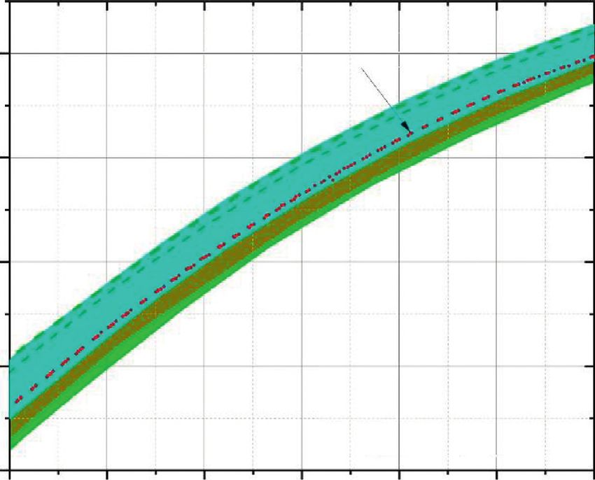

4 Advances in Materials Science and Engineering

 115%∗ measured data
 110%∗ measured data
 105%∗ measured data
 Measured data
 95%∗ measured data
 90%∗ measured data
 Complex modulus (Pa)

 68.3% of data
 85%∗ measured data

 95.5% of data

 99.7% of data
 Extend the original data with different
 coefficients of variation (CoV)
 ∗ Not to scale
 –3SD –2SD –SD Mean –1SD –2SD –3SD
 Value distribution of model parameters

 Log reduced frequency (Hz)
 (a) (b)

 Figure 2: Qualify the data variation and modeling uncertainty quantitatively. (a) Data variation. (b) Modeling uncertainty.

 Xi � xli , xui . (5) Accordingly, the single master curve is extended to a
 master-curve band. Using a generalized sigmoidal model,
 Based on equation 5, the parameter vector x can be the master-curve band can be induced as the two following
extended to data space U, as expressed in the following equations:
equation:
 U � X|xi ε xli , xui , i � 1, 2, 3, 4, . . . , n . (6)

 ⎪
 ⎧
 ⎪ ⎪
 ⎫
 ⎪
 ⎪
 ⎨ αi ⎪
 ⎬
 MCB � ⎪S|Si � δi + , i � 1, 2, 3, 4, . . . , ∞⎪, (7)
 ⎪
 ⎪ ( βi +ci {log(2πf)})
 (1/λi ) ⎪
 ⎪
 ⎩ 1 + λi e ⎭

 αi , βi , δi , ci , λi ∈ U, i � 1, 2, 3, 4, . . . , ∞. (8)

2.5. Procedure to Construct the Master-Curve Band. This band is generated by performing a calculating experiment
section explained how to draw a master-curve band step by using MATLAB code. All possible values in data space U are
step, as shown in Figure 3. After the rheological test, considered. Figure 4 illustrates an example of extending
reference temperature was firstly determined. In what from master curve to master-curve band using a generalized
follows, the shift factors are determined based on the WLF sigmoidal model.
or Arrhenius equations. The rheological model’s selection
is subjective, which could be any empirical or mechanical 2.6. Data Collection and Selected Rheological Models.
models. Once the rheological model is determined, model Four kinds of bitumen were subjected to DSR measurements
parameters can be obtained by solving the target mini- to obtain rheological data. Two of them were unaged and
mization function. The measured isochronal plots are unmodified bitumen, marked as U15 and U70. The numbers
multiplied by the coefficients from 85% to 115% for the following “U” indicated the penetration grade. One bitumen
master-curve band construction. In total, six other groups was the aged U15, noted as A15. The other one was the SBS
of isochronal plots are calculated. modified bitumen based on U70, coded as SBS. All the
 The normal distribution fit is then performed separately samples were subjected to the DSR frequency sweep fol-
at 85%, 90%, and 95% confidence levels. The data space U in lowing the standard procedure.
equation 6 for each parameter is obtained at a specific Two rheological models were used to construct the
confidence level. According to equation 7, the master-curve master-curve band: generalized sigmoidal model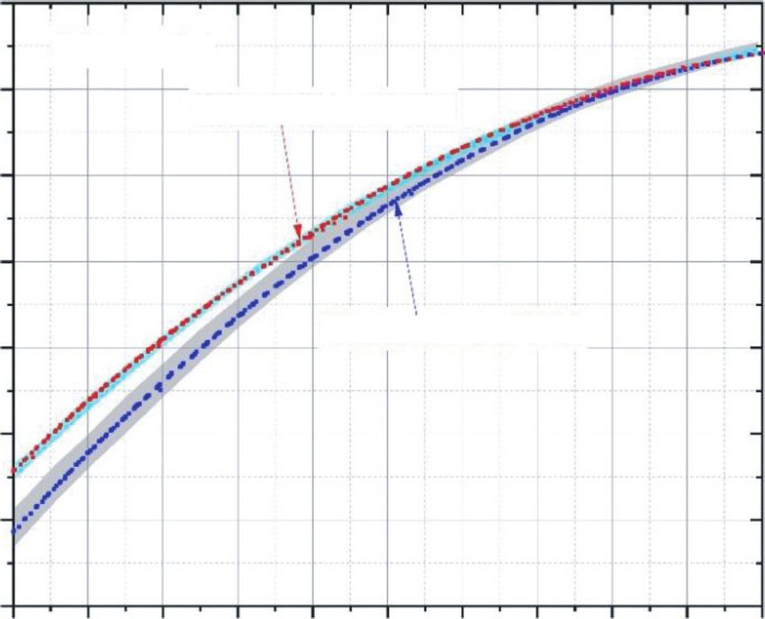

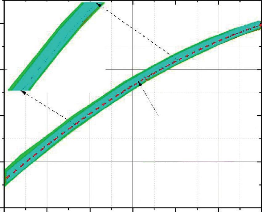
Advances in Materials Science and Engineering 5

 Rheological test

 Multiply original
 Determine Tref
 data

 Calculate shift
 factors

 Select rheological
 model

 Model parameters Curve fitting Master curve

 Normal
 Curve generation
 distribution fit

 Parameter Master curve
 intervals band

 Figure 3: Schematic of master-curve band construction.

 Generalized sigmoidal model
 68.3% of data
 log G∗ = δ + α/[1 + λe (β + γ (log 2πf ))]1/λ
 95.5% of data

 99.7% of data

 1.E + 10
 Master-curve band with –3SD –2SD –SD Mean –1SD –2SD –3SD
 different confidence levels Value distribution of model parameters
 1.E + 09 ∗ Not to scale

 1.E + 08
 Data space
 Complex modulus (Pa)

 U
 1.E + 07

 1.E + 06

 α – 3SD α α + 3SD γ – 3SD γ γ + 3SD
 1.E + 05

 1.E + 04
 δ – 3SD δ δ + 3SD

 1.E + 03
 1.E – 05 1.E – 03 1.E – 01 1.E + 01 1.E + 03 1.E + 05 1.E + 07 1.E + 09
 Reduced frequency (Hz)

 λ – 3SD λ λ + 3SD β – 3SD β β + 3SD

 Figure 4: Extension from master curve to MCBs (example: generalized sigmoidal model).

(introduced above, GS) and CAM model. According to a The CAM model is mathematically represented as fol-
previous study, bitumen’s theoretical glassy modulus is lows [31]:
supposed to be 1 GPa (shear test). Therefore, the CAM ∗ ω υ − (w/υ)
model was utilized in two ways. One refers to the CAM G � Gg 1 + c , (9)
 ω
model with the glassy modulus fixed at 1 GPa. The other one
with the glassy modulus unfixed was noted as CAM (Gg ) where Gg represents the glassy modulus, ωc is the crossover
model. frequency, and υ and w are model parameters.

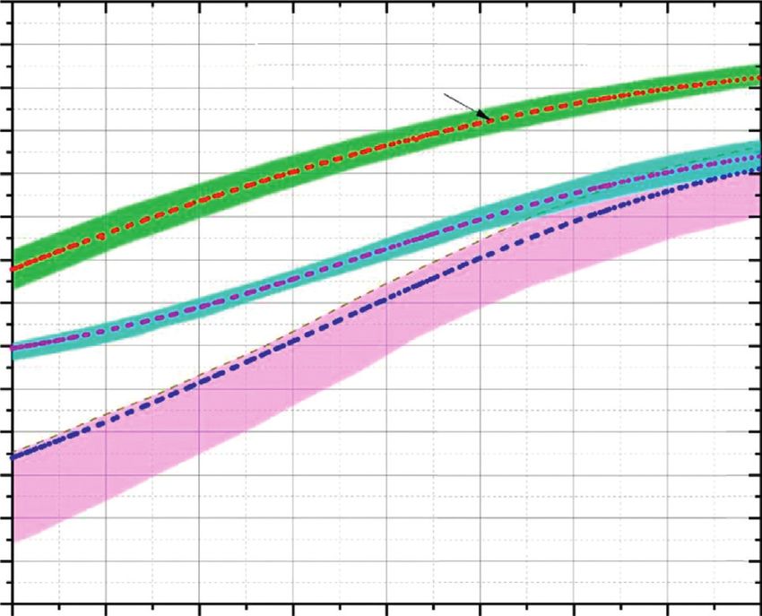
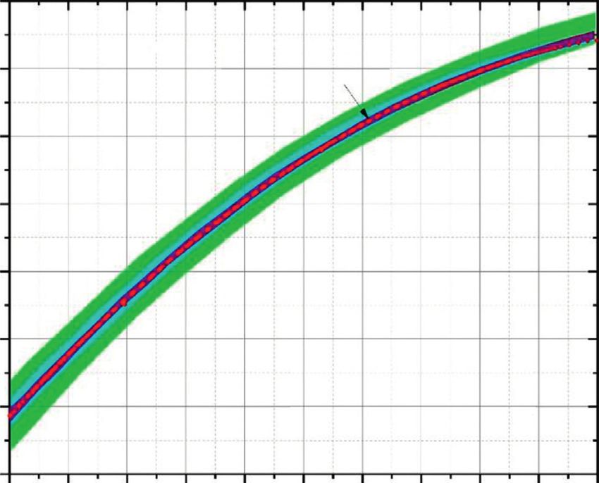
6 Advances in Materials Science and Engineering

3. Basic Properties of the Master-Curve Band 9

The master-curve band is conceptualized by incorporating 8 Constructed master curve
the measurement and/or modeling uncertainty into the

 Log complex modulus (Pa)
master curve. However, very few previous studies intro- 7
duced the master-curve band as well as the basic properties
of the master-curve band. Besides, the rheological model’s 6
effect on the master-curve band is still unknown. The basic
properties varied with different confidence levels and the 5
bitumen types are vague. Therefore, this section discusses the
basic properties of the master-curve band regarding the 4
effect of rheological models, bitumen types, confidence
intervals, and bitumen aging, respectively. 3

 2
3.1. Effect of Rheological Models. Figure 5 presents the –5 –4 –3 –2 –1 0 1 2 3 4 5
master-curve bands of bitumen U15 constructed using three Log reduced frequency (Hz)
different models at a 95% confidence level. It can be seen
that, despite using the same data, different models can result U15_GS_95%
 U15_CAM_95%
in different master-curve bands. The generalized sigmoidal
 U15_CAM(Gg)_95%
model showed the widest band, followed by the CAM and
CAM (Gg ) models. It indicates that the CAM (Gg ) model Figure 5: Master-curve bands constructed using different models.
performed the best in modeling U15 as the least deviation
caused by modeling. The only difference between CAM and
CAM (Gg ) models rests on whether the glassy modulus was showed the smallest sensitivity to the data variation.
fixed. However, the CAM model, which has one parameter Provided that an identical measurement variation oc-
less than the CAM (Gg ) model, showed a wider band. It curred, the master curve of modified bitumen could present
indicates that the fix of the glassy modulus would change the the smallest deviation to the correct master curve. Simi-
values of other parameters. In this sense, the CAM model larly, hard and unmodified bitumen showed less deviation
and CAM (Gg ) model are essentially two different models. compared to softer and unmodified bitumen in this study.
Table 1 presents the parameter intervals calculated at a To further explain the sensitivity of bitumen to rheological
confidence level of 95%. It can be seen that the GS model models, the confidence intervals for different bitumen are
owns five model parameters, which contributed to its wider presented in Table 2. For U15, as the confidence level in-
master-curve band. Although the CAM model has only three creased, the interval was enlarged except for the parameter c.
model parameters, the interval of wc was from 17.61 to 28.32, It indicated that the parameter c is relatively stable when
while in the CAM (Gg ) model the value was only from 1.23 using the GS model to construct U15 even in the presence of
to 1.42. Therefore, it is not true that the band width solely data variation. However, for other parameters, data variation
depends on the number of model parameters. Parameter could result in a change of parameter value.
interval is another critical factor that influences the width of In terms of U70, the model parameters can be divided
the master-curve band. into two groups. The first group (active group), including δ,
 On the other hand, it can be concluded that v and w are α, and λ, complied with the tendency found in U15. The
two model parameters that will not significantly change due other group (including β and c) is the inert group, in which
to data variation. In this study, parameters with such kind of the interval remained almost unchanged as the confidence
character are called inert parameters. In contrast, parameters level increased. In this case, two model parameters would
with a considerable change due to data variation are called not be significantly altered due to the data variation.
active parameters. The inert and active parameters can be Nevertheless, the variation of U70 between the lower and
distinguished by calculating the variation coefficient with a upper values is relatively more considerable than that of
cut-off value of 20%. In this case, the numbers of active U15, which is ascribed to a wider master-curve band. In the
parameters in the GS, CAM (Gg ), and CAM models are four, case of SBS, the parameter λ was also classified into the inert
two, and one, respectively. group. However, the parameter interval in the active group
 was the smallest compared to that of U70 or U15.
 It can be concluded that the model sensitivity of bitumen
3.2. Effect of Bitumen Types. Figure 6 shows the master- is correlated with not only the type of rheological model but
curve bands of different bitumen binders using the GS also the type of bitumen.
model at a 95% confidence level. Various bitumen binders
responded differently to the identical construction pro-
cedure of master-curve bands. As shown in Figure 6, the 3.3. Effect of Confidence Levels. Figure 7 presents the MCBs
MCB of U70 showed the widest band, followed by U15 and of U15 constructed at different confidence levels. When the
SBS. The band width reflects the model sensitivity of bi- rheological model was the GS model, the increase of con-
tumen. Herein, modified bitumen investigated in this study fidence level increased MCB width. As the confidence level

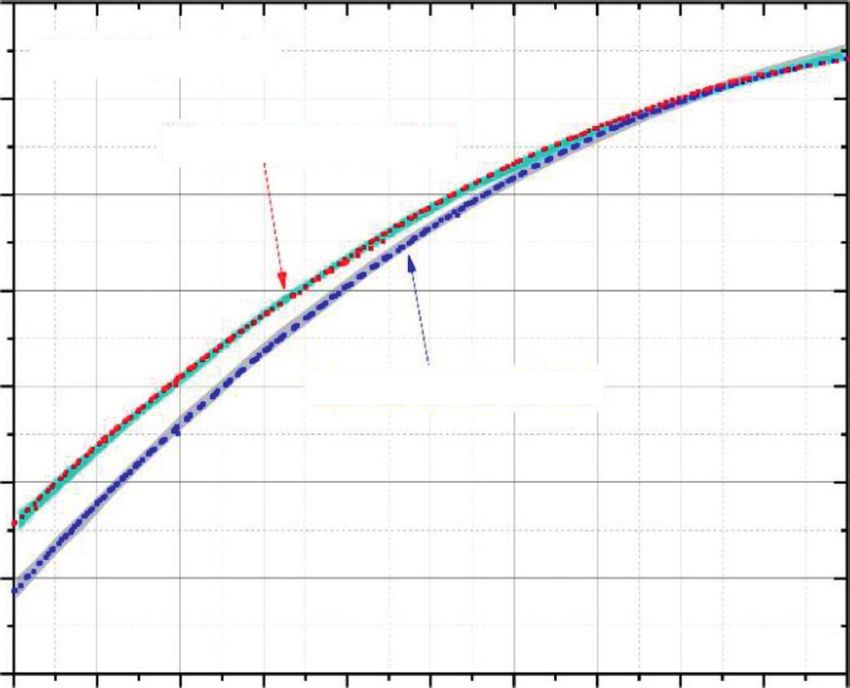
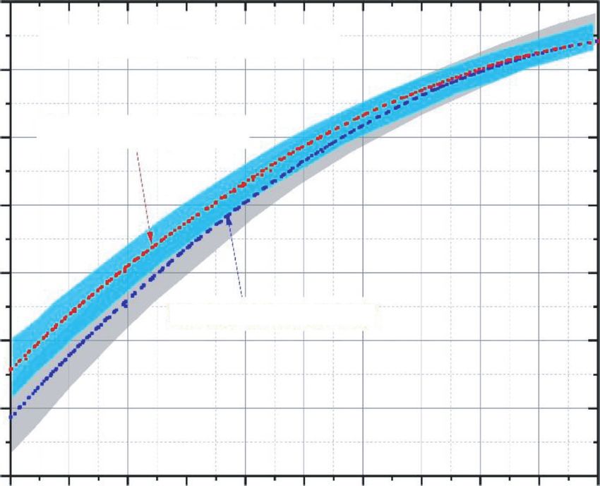
Advances in Materials Science and Engineering 7

 Table 1: Estimated parameter intervals of U15 at confidence level 95%.
 GS model CAM (Gg ) model CAM model
 δ α λ β c Gg (GPa) wc v w wc v w
Lower 10.09 − 11.37 3.52 2.18 0.57 1.95 1.23 0.12 1.22 17.61 0.15 1.01
Upper 10.32 − 10.59 3.66 2.46 0.58 2.46 1.42 0.12 1.23 28.32 0.16 1.05

 10
 9
 8 Constructed master curve
 7
 Log complex modulus (Pa)

 6
 5
 4
 3
 2
 1
 0
 –1
 –2
 –3
 –4
 –4 –3 –2 –1 0 1 2 3 4
 Log reduced frequency (Hz)

 U15_GS_95%
 U70_GS_95%
 SBS_GS_95%
 Figure 6: Master-curve bands of different bitumen binders.

 Table 2: The confidence interval constructed for different bitumen using the GS model.
 95% 90% 85%
Bitumen type Confidence level
 Lower Upper Lower Upper Lower Upper
 δ 10.09 10.32 10.12 10.28 10.13 10.27
 α − 11.37 − 10.59 − 11.24 − 10.72 − 11.21 − 10.75
U15 λ 3.52 3.66 3.55 3.64 3.55 3.63
 β 2.18 2.46 2.23 2.41 2.24 2.40
 c 0.57 0.58 0.57 0.57 0.57 0.57
 δ − 7.06 − 5.33 − 6.92 − 5.47 − 6.83 − 5.56
 α 13.06 14.38 13.17 14.27 13.24 14.20
U70 λ 2.57 4.37 2.71 4.23 2.81 4.13
 β 0.00 0.14 0.01 0.12 0.01 0.12
 c − 0.56 − 0.42 − 0.55 − 0.43 − 0.54 − 0.44
 δ 0.96 1.15 0.98 1.13 0.99 1.12
 α 6.16 6.56 6.19 6.53 6.21 6.51
SBS λ 0.62 0.69 0.63 0.69 0.63 0.68
 β 0.15 0.20 0.15 0.20 0.16 0.20
 c − 0.42 − 0.38 − 0.41 − 0.38 − 0.41 − 0.38

increased, the confidence interval of model parameters utilization of the CAM and CAM (Gg ) models would not
correspondingly grew. However, in the CAM and CAM (Gg ) significantly change the final constructed master curve. This
models, MCB width change with the increase of confidence modeling stability, to some extent, can alleviate the modeling
level was not significant. It illustrated that although the uncertainty of the master curve.
confidence level was altered, the constructed master-curve Nevertheless, this finding brings about some other issues
bands were not sensitive to the change of confidence level. In when comparing master curves between similar bitumen
this condition, given that a modeling error existed, the types. Assuming that bitumen was aged insignificantly, the

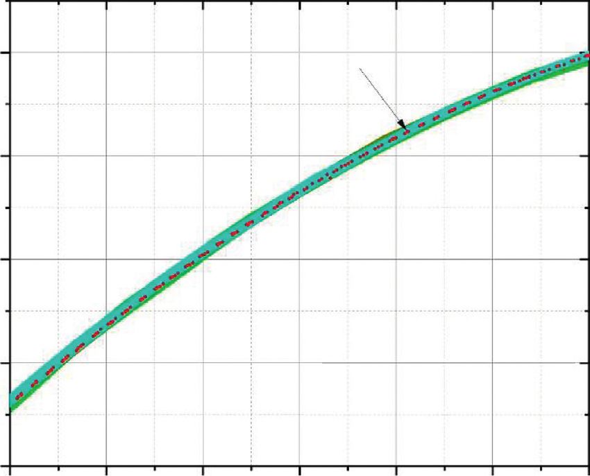
8 Advances in Materials Science and Engineering

 8 8 Constructed master curve
 Log complex modulus (Pa)

 Log complex modulus (Pa)
 7 7

 6 6
 Constructed master curve

 5 5

 4 4
 –3 –2 –1 0 1 2 3 –3 –2 –1 0 1 2 3
 Log reduced frequency (Hz) Log reduced frequency (Hz)

 U15_CAM_95% U15_CAM (Gg)_95%
 U15_CAM_90% U15_CAM (Gg)_90%
 U15_CAM_85% U15_CAM (Gg)_85%
 (a) (b)

 8 Constructed master curve
 Log complex modulus (Pa)

 7

 6

 5

 4
 –3 –2 –1 0 1 2 3
 Log reduced frequency (Hz)
 U15_GS_95%
 U15_GS_90%
 U15_GS_85%
 (c)

Figure 7: Master-curve bands constructed with different confidence levels. (a) CAM model. (b) CAM (Gg) model. (c) Generalized sigmoidal
model.

master curve of aged bitumen was similar to its origin bi- existed. Therefore, the overlapped area claimed the possi-
tumen. In this condition, the master-curve comparison bility that the master curves of A15 and U15 were close to
cannot reveal the essential variation caused by aging, con- each other. In this case, the effect of aging on rheological
sidering the modeling uncertainty. properties of bitumen might be enervated. Therefore, it is
 not appropriate for researchers to identify the aging effect
 using a generalized sigmoidal model to model uncertainty.
3.4. Effect of Bitumen Aging. Figure 8 compares the master- As can be seen from Figures 8(b) and 8(c), the over-
curve bands of unaged and aged bitumen (U15 and A15) lapping area of master-curve bands for A15 and U15 can be
using different rheological models. When the rheological considerably reduced using the CAM or CAM (Gg ) models.
model was selected as the generalized sigmoidal model, the It can be found that the overlapping area was relevant to the
master-curve band of A15 overlapped with U15, especially at master-curve band’s width. As aforementioned, bitumen
high frequencies. The master-curve band refers to all pos- showed the smallest sensitivity to the CAM (Gg ) model.
sible constructed master curves if modeling uncertainty Therefore, the width of the master-curve band tended to

Advances in Materials Science and Engineering 9

 9 9
 Generalized sigmoidal model CAM model
 8 8
 Master curve of A15
 Log complex modulus (Pa)

 Log complex modulus (Pa)
 7 Master curve of A15 7

 6 6

 Master curve of U15
 5 5
 Master curve of U15
 4 4

 3 3

 2 2
 –5 –4 –3 –2 –1 0 1 2 3 4 5 –5 –4 –3 –2 –1 0 1 2 3 4 5
 Log reduced frequency (Hz) Log reduced frequency (Hz)
 (a) (b)
 9
 CAM (Gg) model
 8
 Master curve of A15
 Log complex modulus (Pa)

 7

 6

 5 Master curve of U15

 4

 3

 2
 –5 –4 –3 –2 –1 0 1 2 3 4 5
 Log reduced frequency (Hz)
 (c)

Figure 8: Master-curve band comparison between unaged and aged bitumen. (a) Generalized sigmoidal model. (b) CAM model. (c) CAM
(Gg) model.

present in a small value. A small value of band width in- separately relative to the measurement error and modeling
dicated a small deviation caused by the modeling uncer- uncertainty. For the measurement error, the coefficient of
tainty. Hence, it can be concluded that the modeling variation was used to describe the error quantitatively. The
uncertainty can be eliminated as much as possible if an normal distribution fitting was adopted to obtain the pa-
appropriate rheological model is used. In previous studies of rameter intervals at a specific confidence level for the
rheological modeling of bitumen binders, only the goodness modeling uncertainty. Consequently, the master-curve band
of fit was concerned. The introduction of master-curve can be generated through a calculating experiment via
bands revealed that the rheological model’s selection should MATLAB. Through investigating the fundamental proper-
consider satisfying fitting results and the resistance ability to ties of the master-curve band, some critical findings were
the modeling uncertainty. concluded as follows:
 (1) Ignorance of modeling uncertainty in the estimation
4. Conclusion and Outlook of aging or modification would possibly hinder an
4.1. Conclusion. In the engineering field, measurement and appropriate conclusion to be achieved, especially
modeling uncertainty represent a critical topic. However, when the aging or modification degree is relatively
there is a lack of studies considering the uncertainty in the small.
construction of the master curve. For this reason, this study (2) Master-curve bands constructed for the same bitu-
proposed a method to conclude the uncertainty property. men were different on account of various rheological
The fundamental technology includes two parts, which are models. The width of the master band is dominated

10 Advances in Materials Science and Engineering

 by the sensitivity of bitumen to the rheological German Research Foundation (O.E. 514/10-1). The authors
 model. also gratefully acknowledge financial support from the
 (3) The sensitivity of bitumen to rheological models was China Scholarship Council (CSC no. 201706710009).
 determined by two factors. The first is the number of
 active parameters in the selected rheological model. References
 The second is related to the confidence interval of
 active parameters. [1] Y. Gao, Y. Zhang, F. Gu, T. Xu, and H. Wang, “Impact of
 minerals and water on bitumen-mineral adhesion and
 (4) In this study, the generalized sigmoidal model debonding behaviours using molecular dynamics simula-
 showed the widest master-curve band, while the tions,” Construction and Building Materials,
 CAM (Gg ) model performed the best. Therefore, it is vol. 1711016 pages, 2018.
 recommended to use the CAM (Gg ) model rather [2] Y. Gao, Y. Zhang, Y. Yang, J. Zhang, and F. Gu, “Molecular
 than the generalized sigmoidal model to analyze the dynamics investigation of interfacial adhesion between oxi-
 aging effect. dised bitumen and mineral surfaces,” Applied Surface Science,
 vol. 4791292 pages, 2019.
 [3] S. Wu, Q. Liu, J. Yang, R. Yang, and J. Zhu, “Study of adhesion
4.2. Outlook. It is undeniable that this proposed method between crack sealant and pavement combining surface free
could not be an efficient approach to characterize the energy measurement with molecular dynamics simulation,”
master-curve construction’s uncertainty information. This Construction and Building Materials, vol. 240, Article ID
study’s primary purpose is to introduce uncertainty into the 117900, 2020.
 [4] Y. Gao, L. Li, and Y. Zhang, “Modeling crack propagation in
master curve to strengthen the reliability of the master curve.
 bituminous binders under a rotational shear fatigue load
It is believed that much work should be done to modify the using pseudo j-integral paris’ law,” Transportation Research
master-curve band toward an efficient and thoughtful ap- Record: Journal of the Transportation Research Board,
proach to include the uncertainty information in the master vol. 2674, no. 1, pp. 94–103, 2020.
curve. From the evaluation of the authors, the master-curve [5] Z. Zhang, Q. Liu, Qi Wu, H. Xu, P. Liu, and M. Oeser,
band can be modified from the following perspectives: “Damage evolution of asphalt mixture under freeze-thaw
 cyclic loading from a mechanical perspective,” International
 (1) Notably, a detailed standard procedure to construct Journal of Fatigue, vol. 142, Article ID 105923, 2021.
 the master-curve band was not recommended. The [6] E. Masad, C.-W. Huang, G. Airey, and A. Muliana, “Non-
 reason is that limited types of bitumen and rheo- linear viscoelastic analysis of unaged and aged asphalt
 logical models were investigated in this study. binders,” Construction and Building Materials, vol. 22, no. 11,
 Therefore, an investigation with more samples and pp. 2170–2179, 2008.
 models is expected to validate some arguments in [7] Q. Liu, J. Wu, X. Qu, C. Wang, and M. Oeser, “Investigation of
 constructing the master-curve band. In addition, bitumen rheological properties measured at different rhe-
 more potential influence factors of the master-curve ometer gap sizes,” Construction and Building Materials,
 band will need to be discussed. vol. 265, Article ID 120287, 2020.
 [8] G. D. Airey, “Use of black diagrams to identify inconsistencies
 (2) The coefficient of variation used in this study was based in rheological data,” Road Materials and Pavement Design,
 on the RILEM research. However, it will be more vol. 3, no. 4, pp. 403–424, 2002.
 rational when the coefficient of variation is determined [9] D. I. Alhamali, J. Wu, Q. Liu et al., “Physical and rheological
 by repeatedly conducting the DSR measurements. characteristics of polymer modified bitumen with nanosilica
 (3) Normal distribution fitting was adopted to feature particles,” Arabian Journal for Science and Engineering,
 vol. 41, no. 4, pp. 1521–1530, 2016.
 the modeling uncertainty, and all the parameters
 [10] P. Ahmedzade, A. Fainleib, T. Günay, and O. Grygoryeva,
 were assumed to be independent of each other. “Modification of bitumen by electron beam irradiated recy-
 However, the data space of model parameters can be cled low density polyethylene,” Construction and Building
 established by other advanced uncertainty analysis Materials, vol. 69, pp. 1–9, 2014.
 methods. [11] G. King, M. Anderson, D. Hanson, and P. Blankenship,
 “Using black space diagrams to predict age-induced crack-
Data Availability ing,” in Proceedings of the 7th RILEM International Conference
 on Cracking in Pavements, Dordrecht, Netherlands, August
The data used to support the findings of this study are in- 2012.
cluded within the article. [12] Benedetto, Herve Di, F. Olard, C. . Sauzéat, and B. Delaporte,
 “Linear viscoelastic behaviour of bituminous materials: from
 binders to mixes,” Road Materials and Pavement Design,
Conflicts of Interest vol. 5, no. 1, pp. 163–202, 2004.
 [13] S. Mangiafico, H. Di Benedetto, C. Sauzéat, F. Olard,
The authors declare that they have no conflicts of interest. S. Pouget, and L. Planque, “New method to obtain viscoelastic
 properties of bitumen blends from pure and reclaimed asphalt
Acknowledgments pavement binder constituents,” Road Materials and Pavement
 Design, vol. 15, no. 2, pp. 312–329, 2014.
The authors would like to acknowledge the National Natural [14] H. M. Nguyen, S. Pouget, H. di Benedetto, and C. Sauzéat,
Science Foundation of China (no. 52078190) and the “Time-temperature superposition principle for bituminous

Advances in Materials Science and Engineering 11

 mixtures,” Revue européenne de génie civil, vol. 13, no. 9, [30] T. O. Medani, M. Tech, and M. Huurman, “Constructing the
 pp. 1095–1107, 2009. stiffness master curves for asphaltic mixes,” Civil Engineering,
[15] N. I. Nur, E. Chailleux, and G. D. Airey, “A comparative study vol. 25, no. 12, pp. 1813–1821, 2003.
 of the influence of shift factor equations on master curve [31] N. Yusoff Nur Izzi, F. M. Jakarni, V. H. Nguyen, M. R. Hainin,
 construction,” International Journal of Pavement Research and G. D. Airey, “Modelling the rheological properties of
 and Technology, vol. 4, no. 6, pp. 324–336, 2011. bituminous binders using mathematical equations,” Con-
[16] F. P. Germann and R. L. Lytton, “Methodology for predjcting struction and Building Materials, vol. 40, pp. 174–188, 2013.
 the reflection cracking life of asphalt concrete overlays,” Texas
 A&M Transportation Institute, Austin, TX, USA, Res. Rpt.
 No. 207-5, 1979.
[17] L. Francken and C. Clauwaert, “Characterization and struc-
 tural assessment of bound materials for flexible road struc-
 tures,” in Proceedings of the 6 International Conference on
 Asphalt Pavements, pp. 130–144, Ann Arbor, MS, USA,
 August 1987.
[18] M. Williams and D. Ferry, “The temperature dependence of
 relaxation mechanisms in amorphous polymers and other
 glass-forming liquids,” Journal of the American Chemical
 Society, vol. 77, no. 14, pp. 3701–3707, 1955.
[19] T. K. Pellinen, M. W. Witczak, and R. F. Bonaquist, “Asphalt
 mix master curve construction using sigmoidal fitting func-
 tion with non-linear least squares optimization,” Geotechnical
 Special Publication, vol. 2576 pages, 2004.
[20] M. Yusoff Nur Izzi, M.-S. Ginoux, G. Dan Airey, and M. Rosli
 Hainin, “Modelling the linear viscoelastic rheological prop-
 erties of base bitumens,” Malaysian Journal of Civil Engi-
 neering, vol. 22, no. 1, 2010.
[21] E. Chailleux, R. Guy, C. Such, and C. De La Roche, “A
 mathematical-based master-curve construction method ap-
 plied to complex modulus of bituminous materials,” Road
 Materials and Pavement Design, vol. 7, no. 1, 2006.
[22] M. Yusoff Nur Izzi, M. T. Shaw, and G. D. Airey, “Modelling
 the linear viscoelastic rheological properties of bituminous
 binders,” Construction and Building Materials, vol. 25, no. 5,
 pp. 2171–2189, 2011.
[23] J. Carswell, M. J. Claxton, and P. J. Green, “Dynamic shear
 rheometers: making accurate measurements on bitumens,” in
 Proceedings of Conference of the Australian Road Research
 Board, pp. 219–237, Canberra. Australia, August 1998.
[24] J. Wu, M. Y. Nur Izzi, F. Mohd Jakarni, and M. Rosli Hainin,
 “Correction of compliance errors in the dynamic shear
 modulus of bituminous binders data,” Sains Malaysiana,
 vol. 42, no. 6, pp. 783–792, 2013.
[25] M. N. Partl and H. Bahia, Advances in Interlaboratory Testing
 and Evaluation of Bituminous Materials: State-Of-The-Art
 Report of the RILEM Technical Committee 206-ATB, Springer
 Science & Business Media, Berlin, Germany, 2012.
[26] N. I. Nur, D. Mounier, G. Marc-Stéphane, M. Rosli Hainin,
 G. D. Airey, and Hervé Di Benedetto, “Modelling the rheo-
 logical properties of bituminous binders using the 2S2P1D
 model,” Construction and Building Materials, vol. 38,
 pp. 395–406, 2013.
[27] R. de Carteret, C. Lee, J. Metcalf, and J. Rebbechi, Guide to
 Pavement Technology: Part 8: Pavement Construction Indian,
 Academy of Sciences, Bengaluru, Karnataka, India, 2009.
[28] S. M. Asgharzadeh, N. Tabatabaee, K. Naderi, M. Partl, and
 M. Partl, “An empirical model for modified bituminous
 binder master curves,” Materials and Structures, vol. 46, no. 9,
 pp. 1459–1471, 2013.
[29] D. Wang, Q. Liu, Q. Yang, C. Tovar, Y. Tan, and M. Oeser,
 “Thermal oxidative and ultraviolet ageing behaviour of nano-
 montmorillonite modified bitumen,” Road Materials and
 Pavement Design, vol. 22, no. 1, pp. 121–139, 2019.