Latent Pose Estimator for Continuous Action Recognition
←
→
Page content transcription
If your browser does not render page correctly, please read the page content below
Latent Pose Estimator for Continuous Action
                    Recognition

        Huazhong Ning1 , Wei Xu2 , Yihong Gong2 , and Thomas Huang1 ,
                    1
                        ECE, U. of Illinois at Urbana-Champaign, USA
                              {hning2,huang}@ifp.uiuc.edu
                          2
                            NEC Laboratories America, Inc., USA
                               {xw,ygong}@sv.nec-labs.com

       Abstract. Recently, models based on conditional random fields (CRF)
       have produced promising results on labeling sequential data in several
       scientific fields. However, in the vision task of continuous action recog-
       nition, the observations of visual features have dimensions as high as
       hundreds or even thousands. This might pose severe difficulties on para-
       meter estimation and even degrade the performance. To bridge the gap
       between the high dimensional observations and the random fields, we
       propose a novel model that replace the observation layer of a traditional
       random fields model with a latent pose estimator. In training stage, the
       human pose is not observed in the action data, and the latent pose esti-
       mator is learned under the supervision of the labeled action data, instead
       of image-to-pose data. The advantage of this model is twofold. First, it
       learns to convert the high dimensional observations into more compact
       and informative representations. Second, it enables transfer learning to
       fully utilize the existing knowledge and data on image-to-pose relation-
       ship. The parameters of the latent pose estimator and the random fields
       are jointly optimized through a gradient ascent algorithm. Our approach
       is tested on HumanEva [1] – a publicly available dataset. The experi-
       ments show that our approach can improve recognition accuracy over
       standard CRF model and its variations. The performance can be further
       significantly improved by using additional image-to-pose data for train-
       ing. Our experiments also show that the model trained on HumanEva
       can generalize to different environment and human subjects.

1    Introduction
Recognizing human actions in videos with natural environments provides an in-
frastructure for a wide range of applications spanning visual surveillance, systems
for entertainment, human-computer interfaces, and so on. It is a specific example
of a widely studied problem of sequence labeling that arises in several scientific
fields. A well understood and widely used probabilistic model for this problem is
Hidden Markov Model (HMM) [2]. But HMMs make strict assumption that ob-
servations are conditionally independent given class labels, and cannot represent
multiple interacting features and long-range dependencies of the observations.
Thus, it largely limits the applicability of the HMM models.

D. Forsyth, P. Torr, and A. Zisserman (Eds.): ECCV 2008, Part II, LNCS 5303, pp. 419–433, 2008.

c Springer-Verlag Berlin Heidelberg 2008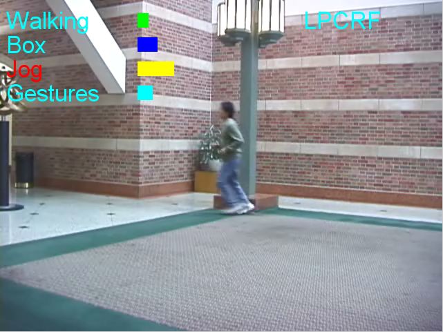
420     H. Ning et al.

   Conditional random fields models [3] relax the assumption of observation in-
dependency and has exhibited success to discriminate actions in both segmented
and unsegmented video sequences [4,5]. In [4], a latent-dynamic conditional ran-
dom field (LDCRF) model is proposed to capture both extrinsic dynamics and
intrinsic structure of head and gaze aversion gestures. The poses of 3D head or
eye gaze are robustly estimated using a view based appearance model, and the
model recognizes the gestures based on the pose representations. However, in
action recognition where articulated human body is involved, the explicit pose
of the body parts could not be reliably estimated by currently existing tracking
algorithms. In other words, it is impractical to use LDCRF to recognize complex
human actions in the same way as in [4]. An possible solution is to directly feed
the visual features (e.g., block SIFT [6] and silhouette[7]), instead of human
poses, to the random fields as in [5] where a chain conditional random fields
(CRF) model [3] is used. But the dimension of visual features is usually as high
as hundreds or even thousands, compared to 10-50 dimensions of human poses,
and their discriminative power to represent human actions is also worse than
human poses. This might increase the complexity of parameter estimation in
random fields while degrade the performance.
   In this paper, we propose a novel model to bridge the gap between the high
dimensional visual features and the random fields. As we know, human pose is
a very compact and informative representation for human images. And recently,
the multi-modal image-to-pose relationship has been successfully exploited using
discriminative models, such as linear/nonlinear regression [7], Bayesian mixture
of experts (BME) [6], and so on. Therefore, we propose a model that replaces
the observation layer of the random fields with an image-to-pose discriminative
model. Fig. 1 illustrates the graphical structure of our model. This image-to-pose
layer learns to convert the high dimensional observations into more compact and
informative representations (such as poses of articulated human body) under the
supervision of labeled action data. We call it latent pose estimator, because it is
not explicitly estimated from labeled image-to-pose data. Actually, the human
poses are not observed in action training data. Of course, additional image-to-
pose data, if available, can also be added to the learning process. In practice,
the output of the latent pose estimator can be human pose (image-to-pose data
are enough) or any other compressed representations (not enough or no pose
data), but we still use the term “pose estimator”. We call our model latent
pose conditional random fields (LPCRF). In this paper, our model is based on
LDCRF, but it can be extended to any other CRF variations. Our experiments
show that the use of latent pose estimator can improve recognition accuracy
over traditional CRF or LDCRF even without using any image-to-pose data for
training.
   The structure of our LPCRF model not only maintains the strength of the
LDCRF model in that it captures both extrinsic dynamics and internal sub-
structure, but also enables the model to recognize actions from high dimensional
visual features without increasing the complexity of the feature functions. Due
Latent Pose Estimator for Continuous Action Recognition        421

                                    z1    z2      zn    z1        z2         zn

                z1    z2      zn    h1   h2       hn    h1        h2         hn

                x1    x2      xn    x1   x2       xn    y1        y2         yn
                                                        Latent pose estimator

                                                        x1        x2         xn
                      CRF                LDCRF               LPCRF (our model)

Fig. 1. Graphical structures of our LPCRF model and two existing models: CRF [3]
and LDCRF [4]. In these models, x is a visual observation, z is the class label (e.g.,
walking or hand waving) assigned to x , and h represents a hidden state of human
actions (e.g., left-to-right/right-to-left walking). The subscripts index the frame num-
ber of the video sequence. In our LPCRF model, the observation layer of the random
fields is replaced with a latent pose estimator that learns to compress the high dimen-
sional visual features x into a compact representation (like human pose) y. Our model
also enables transfer learning to utilize the existing knowledge and data on image-to-
pose relationship. The dashed rectangles means that y’s are technically deterministic
functions of x when the parameters of the latent pose estimator are fixed.

to this advantage, our model can recognize human actions with complex articu-
lations in both segmented and unsegmented video sequences.
   Another advantage of our LPCRF model is that it enables transfer learning
[8] to fully utilize the existing knowledge and data on image-to-pose relationship.
Firstly, our model can be incrementally built on an existing discriminative pose
estimator that is well-trained on either synthetic or real image-to-pose datasets.
More specifically, we use the parameters of an existing pose estimator (if avail-
able) to initialize the latent pose estimator. This allows a growing algorithm
to acquire new knowledge while keeping old knowledge and to reduce the re-
development and learning costs. Secondly, newly available image-to-pose data,
if available, can be naturally added to the learning process to refine the model
parameters without modifying the structure of our model.
   The literature that is closely related to our research includes action recognition
based on either 2D/3D silhouettes [9,10], 2D body configurations [11], motion
trajectories [12], or body kinematics [13]. These works rely on representations of
explicit pose or compact silhouette to recognize actions. These representations
are generated by a fixed component which cannot be adapted to the given task
of action recognition. While in our system, the latent pose estimator is treated
as a trainable feature extractor that can be improved with more action data.
The benefit of adaptation is clearly demonstrated in our experiments.

2    Latent-Dynamic Conditional Random Fields

First, we briefly introduce the LDCRF model[4] that was proposed to solve
the problem of labeling unsegmented video sequences. It incorporates hidden
422 H. Ning et al.
state variables into the traditional CRF [3] to model the sub-structure of human
actions, and combines the strengths of CRFs and HCRFs [14] to capture both
extrinsic dynamics and intrinsic structure.
Given a sequence of observations X = {x1 , x2 , · · · , xn }, the LDCRF model
predicts a sequence of class labels z = {z1 , z2 , · · · , zn }. Each xi is a visual rep-
resentation for i-th frame. Each zi ∈ Z is the class label of frame xi , where
Z is the set of all possible class labels of the concerned actions. To model the
sub-structure of the actions (e.g., left-to-right/right-to-left walking), a sequence
of hidden variables h = {h1 , h2 , · · · , hn } is incorporated into the CRF model.
Fig. 1 illustrates the graphical structure of the h layer in LDCRF. These hid-
den variables are not observed in the training examples, but are instantiated in
the predicting stage. The transitions among them model both the substructure
patterns of individual actions and the external dynamics between actions.
The LDCRF is restricted to have disjoint sets of hidden states associated with
each class label. Denote Hz the set of hidden states for class z, and Hz = {h|hj ∈
Hzj , j = 1 · · · n} the set consisting of all the possible
sequences of hidden states
compatible with the label sequence z. Let H = z Hz all the possible hidden
state sequences. With these definitions, the LDCRF model is defined as
P (z|X, Φ) = P (z|h, X, Φ)P (h|X, Φ) = P (h|X, Φ) (1)
h h∈Hz
where Φ is set of parameters of the model. The second equation is due to the
fact that, by definition, P (z|h, X, Φ) = 1 for any h ∈ Hz , otherwise 0.
Assume the graph for a video sequence is a simple chain. According to the
fundamental theorem of random fields [15], the joint distribution over the hidden
state sequence h given X has an exponential form
⎛ ⎞
1
P (h|X, Φ) = exp ⎝ VΦ (j, hj , X) + EΦ (j, hj−1 , hj , X)⎠ , (2)
KΦ (X, H) j j
where KΦ (X, H) is the observation dependent normalization,
⎛ ⎞
KΦ (X, H) = exp ⎝ VΦ (j, hj , X) + EΦ (j, hj−1 , hj , X)⎠ , (3)
h∈H j j
summarizing over all hidden state sequences in H. And Φ = {λ1 , λ2 , · · · , μ1 , μ2 ,
· · · } is the set of model parameters. VΦ (j, hj , X) and EΦ (j, hj−1 , hj , X) are sum
of feature functions on individual vertex j and edge (j − 1, j), respectively,
VΦ (j, hj , X) = λk sk (j, hj , X), (4)
k
EΦ (j, hj−1 , hj , X) = μk tk (j, hj−1 , hj , X). (5)
k
where sk and tk are feature functions. sk are state functions that depend on
a single hidden variable of a sub-action in the model, and tk are transitionLatent Pose Estimator for Continuous Action Recognition 423
functions that depend on pairs of hidden variables. We also use Vja and Ejab as
short representations of VΦ (j, a, X) and EΦ (j, a, b, X).
3 Latent Pose Conditional Random Fields
Our latent pose conditional random fields (LPCRF) model is a generalization
of CRF and LDCRF. Fig. 1 illustrates its graphical structure. The latent pose
estimator learns to convert an observation vector x into a more compact and
informative representation y, and the model recognizes human actions based
on the pose sequence Y = {y1 , y2 , · · · , yn }. Later we denote the latent pose
estimator as P (y|x, Θ) in probabilistic form or y = Ψ (x, Θ) in deterministic
form, where Θ is the set of parameters of the latent pose estimator and is jointly
optimized with the random fields using a gradient ascent algorithm.
3.1 Formulation of our LPCRF Model
Using the notations and definitions for the LDCRF model in Section 2, our
model is defined as
P (z|X, Ω) = P (z|Y, Φ) = P (h|Y, Φ) (6)
h∈Hz
where Y = Ψ (X, Θ) is the optimal estimation of the latent pose estimator given
observations X and parameters Θ, and Ω = {Φ, Θ} represents all the model
parameters. The joint distribution over the hidden state sequence h given Y still
has an exponential form
⎛ ⎞
1
P (h|Y, Φ) = exp ⎝ VΦ (j, hj , Y ) + EΦ (j, hj−1 , hj , Y )⎠ , (7)
KΦ (Y, H) j j
where KΦ (Y, H) is the observation dependent normalization in Eqn. 3.
If the parameters Θ for the latent pose estimator are fixed, our LPCRF model
collapses into an LDCRF model. If each class label z ∈ Z is constrained to have
only one hidden sub-action, i.e., |Hz | = 1, the LDCRF model further collapses
into a CRF model. Hence, our LPCRF model is a more general framework of
CRF and LDCRF. However, our LPCRF model is essentially different from both
CRF and LDCRF in some aspects. In our model, input features used by the ran-
dom fields are trainable and are jointly optimized with the random fields, while
in CRF and LDCRF, the input features are fixed and cannot be tuned for the
given recognition task. The latent pose estimator encodes the knowledge of mul-
timodal image-to-pose relationship and provides optimal feature representation
for action recognition. This knowledge can be acquired from existing well-trained
models (if available) and adapted for action recognition in the learning process.
In all, the latent pose estimator is seamlessly integrated and globally optimized
with the random fields.424 H. Ning et al.
The model parameters Ω = {Φ, Θ} are learned from training data consisting of
labeled action sequences (X (t) , z(t) ). The labeled image-to-pose data (x(t) , y(t) ),
if available, can also be utilized as auxiliary data. The optimal parameters Ω ∗
is obtained by maximizing the objective function:
1
L(Ω) = log P (z(t) |X (t) , Ω) − 2 Φ2 +η log P (y(t) |x(t) , Θ) (8)
t 2σ t
L (Ω)
2
L1 (Ω) L3 (Ω)
where the first term, denoted as L1 (Ω), is the conditional log-likelihood of the
action training data. The second term L2 (Ω) is the log of Gaussian prior P (Φ) ∼
exp − 2σ1 2 Φ2 with variance σ 2 and it prevents Φ from drifting too much.
And the third term L3 (Ω) is the conditional log-likelihood of the image-to-pose
training data. η is a constant learning rate. Note that our model enables the
image-to-pose data to be naturally added to the learning process.
3.2 The Latent Pose Estimator
The image-to-pose relation is highly non-linear. Fortunately, close observation
of human images shows that human appearance changes very fast as the human
global orientation changes, while the appearance changes relatively slowly in a
fixed orientation. Therefore, we may assume that the image-to-pose distribution
in a fixed orientation can be well modelled by a single or a combination of linear
regressor(s). This leads us to use the Bayesian mixtures of experts (BME) [16]
to model the multi-modal image-to-pose distributions. Suppose x is the visual
feature of the image and y is the human pose, the model with M experts is:
M
p(y|x, Θ) = g(x, νi )p(y|x, Ti , Λi ) (9)
i=1
where
T
eνi x
g(x, νi ) = ν T x (10)
je
j
p(y|x, Ti , Λi ) ∼ N (y; Ti x, Λi ) (11)
Here Θ = {νi , Ti , Λi |i = 1, 2, · · · , M } consists of the parameters of the BME
model. The expert p(y|x, Ti , Λi ) is an Gaussian distribution with mean Ti x and
covariance matrix Λi . The mixing proportions of the experts, g(x, νi ), are input
dependent and work like gates that can competitively switch-on multiple experts
for some input domains, allowing multi-modal conditionals. They can also pick
a single expert for unambiguous inputs by switching-off other experts. Given the
input x and parameters Θ, the optimal pose estimation of the BME model is
M
y∗ = yP (y|x, Θ)dy = g(x, νi )Ti x (12)
i=1Latent Pose Estimator for Continuous Action Recognition 425
The BME model has exhibited success in representing image-to-pose distrib-
utions in the literature [6]. But our LPCRF model is not limited to the BME
representation. We can replace the BME model with any other differentiable
discriminative models without major modifications to our LPCRF structure.
3.3 Learning Model Parameters
We use an iterative gradient ascent algorithm to search for the optimal model
parameters that maximize the objective function, i.e., Ω ∗ = arg maxΩ L(Ω).
At each iteration, Ω can be updated by Ω ← Ω + ξ ∂L(Ω) ∂Ω or any other Quasi-
Newton methods, where ξ is the learning rate. First, we compute ∂L(Ω)/∂Φ for
estimation of Φ.
∂L(Ω)/∂Φ can be obtained by summarizing the gradients of log P (z|X, Ω)
with respect to Φ over all training samples (X, z). According to the chain rule,
the gradient ∂ log P (z|X, Ω)/∂φ for a parameter φ ∈ Φ is
∂ log P (z|X, Ω) ∂ log P (z|X, Ω) ∂Vja ∂ log P (z|X, Ω) ∂Ejab
= + (13)
∂φ j,a
∂Vja ∂φ ∂Ejab ∂φ
j,a,b
Given Eqn. 4 and 5, the gradients ∂Vja /∂φ and ∂Ejab /∂φ are the cor-
responding feature function. And the gradients ∂ log P (z|X, Ω)/∂Vja and
∂ log P (z|X, Ω)/∂Ejab can be expressed in terms of the marginal probabilities
over individual vertex j or edge (j − 1, j),
∂ log P (z|X, Ω)
= P (hj = a|z, Y, Φ) − P (hj = a|Y, Φ) (14)
∂Vja
∂ log P (z|X, Ω)
= P (hj−1 = a, hj = b|z, Y, Φ) − P (hj−1 = a, hj = b|Y, Φ)(15)
∂Ejab
These marginal probabilities can be efficiently calculated using belief propaga-
tion [3] due to the chain structure of the random fields.
Learning the parameters Θ involves computation of ∂L1 (Ω)/∂Θ and, if image-
to-pose training data are available, ∂L3 (Ω)/∂Θ. The gradient ∂L3 /∂Θ is the
sum of the gradients of the BME model that can be found in [16]. To obtain
∂L1 (Ω)/∂Θ, we rely on the chain rule to compute
∂ log P (z|X, Ω) ∂ log P (z|X, Ω) ∂Vja ∂vec(Y )
= (16)
∂Θ j,a
∂Vja ∂vec(Y ) ∂Θ
for specific training sample (X, z). Here, vec(A) is the stacked columns of A, and
Y is the optimal estimation of the latent pose estimator (by Eqn. 12) given X
and current estimation Θ. In Eqn. 16, we assume the transition functions tk are
independent of Y . The gradient ∂Vja /∂vec(Y ) depends on the definition of state
functions. Note that the chain rule decouples the gradient ∂ log P (z|X, Ω)/∂Θ
into three simple factors. The value of the factor ∂ log P (z|X, Ω)/∂Vja has al-
ready been computed by Eqn. 14 in estimation of Φ and is back propagated to426 H. Ning et al.
the latent pose layer for estimation of Θ. The feature functions are entirely iso-
lated into a single factor ∂Vja /∂vec(Y ). And the third factor consists of all the
calculations on the latent pose estimator. Thus, the decoupling allows flexible
deployment of feature functions and latent pose estimator without increasing
the complexity of gradient computations.
Computation of the product of ∂Vja /∂vec(Y ) and ∂vec(Y )/∂Θ is straightfor-
ward. Note that L1 (Ω) does not explicitly depend on the covariance matrixes
of the BME model, i.e., Λi cannot be updated from action data. We use image-
to-pose data (if available) to update Λi , or directly use the Λi of an existing
well-trained BME model, or, if both are not available, just assume constant
covariance matrixes.
3.4 Feature Functions
In our model, the feature functions are differentiable with respect to the latent
poses so that gradient ascent algorithm are applicable. Our feature functions
resemble the well-known logit model and are widely used in the literature [4,3].
We have |H|×|H| transition functions and each corresponds to a hidden variable
pair (h, h ), denoted by thh :
thh (j, hj−1 , hj , Y ) = δ(h, hj−1 )δ(h , hj ). (17)
The corresponding parameters μhh form an |H| × |H| matrix that is essentially
a transition matrix. It models both the external dynamics between actions and
the internal substructures of individual actions [4].
To make the computation tractable, the state functions do not model the
dependency of the entire observation sequence but, instead, depend only on a
window around the current frame. In other words, sk (j, hj , Y ) = sk (j, hj , Ỹj ),
where Ỹj = [yj−w , · · · , yj+w ] is a window around the j-th frame with window
size 2w + 1. Assume yj has dimension d. We have |H|× d(2w + 1) state functions,
and each corresponds to a pair (h, l), where 1 ≤ l ≤ d(2w+1). The state function
shl (j, hj , Y ) = δ(h, hj )Ỹj (l), where Ỹj (l)
is the l-th entry in Ỹj . With
the window
feature, ∂Vja /∂Y is a sparse matrix 0d×(j−w−1) , λ̃a , 0d×(n−j−w) , where λ̃a is
a d × (2w + 1) matrix consisting of the parameters λal corresponding to all sal
for a fixed a ∈ H. Thus, Eqn. 16 can be further simplified.
3.5 Inference
Given the model parameters Ω ∗ learned from the training data, prediction of a
new test sequence X is to estimate the most probable sequence labels z∗ that
maximizes our model
z∗ = arg max P (z|X, Ω ∗ ) = arg max P (z|Y ∗ , Φ∗ ) (18)
z z
where Y ∗ is the optimal pose estimation given X and Θ∗ .Latent Pose Estimator for Continuous Action Recognition 427
The sequence labels z∗ can be estimated using either Viterbi path [3] or mar-
ginal probabilities [4]. We choose the later for this paper. We compute for each
frame i the marginal probabilities P (hi = a|Y ∗ , Φ∗ ) for all a ∈ H. The marginal
probabilities are summed according to the sets of hidden states Hz . The label
zi∗ associated with the set having maximum summed marginal probabilities is
assigned to frame i. As we mentioned in Section 3.3, P (hi = a|Y ∗ , Φ∗ ) can be
efficiently computed using belief propagation. Thus, the inference operation is
also very efficient.
4 Experimental Results
HumanEva dataset. We test the effectiveness of our approach on a real hu-
man motion dataset–HumanEva–made publicly available by the Brown Group
[1]. The dataset was captured simultaneously using a calibrated marker-based
motion capture system and multiple high-speed video capture systems. It con-
tains multiple subjects performing a set of predefined actions with repetitions,
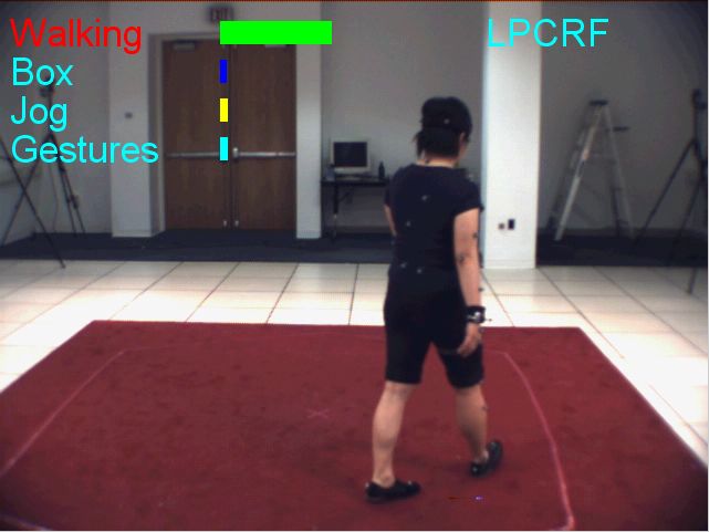
and was originally partitioned into Train, Validate, and Test sub-sets. Fig. 4(a)
(top) gives a sample image. We choose 4 actions1 : Walking, Box, Jog, and Ges-
tures, performed by subjects S1, S2 and S3, captured by cameras C1, C2, and
C3. There are 56,261 video frames in total. Note that our model will recognize
actions under different view points.
The original motion data provided by HumanEva were (x, y, z) locations of
the body parts in the world coordinate system. There is a total of 10 parts: torso,
head, upper and lower arms, and upper and lower legs. In this work, we discard
the internal parameters of the human body model (like limb length), and convert
the (x, y, z) locations to global orientation of torso and relative orientation of
adjacent body parts. Each orientation is represented by 3 Euler angles.
Visual features for image representation. We choose the bag-of-words
model [17] to represent the human images, because it is resistant to a large
misalignment of the human region in the detection window that may pose diffi-
culties to many other representations. For each video frame, the human window
is detected by human detector or background subtraction and is scaled to a
fixed size. In the human window, we extract a set of local descriptors, called
Appearance and Position Context (APC) descriptor [18]. The bag-of-words rep-
resentation of this frame is a 300-bin histogram of the APC descriptors.
Comparison of different models. We run several experiments in order to
compare CRF and LDCRF with our LPCRF model under different configura-
tions. The training data include all videos in both Train and Validate subsets
with 25,645 frames, and the testing data include the videos in the Test subset
with 30,616 frames. The window size w for the feature function is set to 3, i.e.,
the context of observations of 7 frames is explored at current positions. All mod-
els have 4 states, each corresponding to an action class. The number of hidden
1
The ThrowCatch action is not selected, because we failed to extract video frames
from S1 Validate and S3 Train/Validate, and have frequent frame drops in S1 Train
and S2 Train/Validate, even using the tool provided by the HumanEva dataset itself.428 H. Ning et al.
1 1 1
Walking Walking
Box Box
0.8 Jog 0.8 Jog 0.8
Probability of action
Probability of action
Probability of action
Gestures Gestures
0.6 0.6 0.6
0.4 0.4 0.4
Walking
0.2 0.2 0.2 Box
Jog
Gestures
0 0 0
0 100 200 300 400 500 600 700 800 900 0 100 200 300 400 500 600 700 800 900 0 100 200 300 400 500 600 700 800 900
Frame number Frame number Frame number
(a) CRF (b) LDCRF (c) LP CRFpure
Fig. 2. Probability of actions on sequence S2 Box Test C3. Both CRF (a) and LD-
CRF (b) have much uncertainty in labeling this sequence, achieving recognition rate of
69.5% and 70.5%, respectively. Our LP CRFpure model (c) significantly improves the
recognition rate to 85.6%, even without using pose knowledge. Best viewed in color.
states for each action class is chosen as 3 for both LPCRF and LDCRF. We use
5 experts for the BME model. In testing, each video frame is labelled as one of
the 4 actions that has maximum marginal probabilities. Here, the recognition
rate is computed based on frames, not on sequences, because each sequence is
very long and this metric is also appropriate for unsegmented sequences.
Our LPCRF model is tested under 4 configurations. 1) LP CRFinit : the para-
meters Θ of the latent pose estimator are initialized using the parameters of an
existing BME model that is well-trained on 5,000 frames randomly selected from
the Train subset, and then are further updated iteratively on action videos. 2)
LP CRFf ix : Θ are initialized using the same BME model but are fixed in the
learning process. Essentially, it is an LDCRF trained on pose sequences that
are obtained by an existing BME model. 3) LP CRFxy : the model is randomly
initialized, but uses training data including both action videos and 1,000 extra
image-to-pose pairs selected from the Train subset. 4) LP CRFpure : it is also
randomly initialized but trained purely on action data, i.e., it does not utilize
image-to-pose knowledge and data, and uses a setup as CRF and LDCRF.
In Table 1, Figs. 2, ??, and 3, we analyze the the performance of the six
models. Table 1 gives the confusion matrixes and average recognition rates of
these models. From them, we note that: 1) The LP CRFpure outperforms CRF
and LDCRF without using any pose-to-image data. This demonstrates the ef-
fectiveness using a trainable feature extractor to compress the high dimensional
observations into more informative and compact feature vectors. This trainable
feature extractor decreases the complexity of the random fields, and, in turn,
increases the performance. 2) With additional image-to-pose data, LP CRFinit
and LP CRFxy achieve the best performance, which demonstrates that our
model effectively transfers the knowledge on image-to-pose relationship to the
new vision task of action recognition. 3) LP CRFf ix is essentially a LDCRF but
it outperforms the latter. It concludes that the estimated human poses, com-
pared with the original visual features, are more powerful in action recognition.
4) LP CRFinit achieves a higher performance than LP CRFf ix , although both
are initialized by the same BME model. This means that further updating of theLatent Pose Estimator for Continuous Action Recognition 429
Table 1. Confusion matrixes of six models. The last row of each table gives model name
and the average recognition rate. LP CRFinit achieves the best performance 95.0%.
wlk box jog gest wlk box jog gest wlk box jog gest
wlk 95.0 0.1 4.9 0 96.3 0 3.7 0 97.8 0 0.2 2.0 wlk
box 0.4 79.4 10.9 9.3 0 75.0 16.2 8.8 0.9 92.5 5.8 0.8 box
jog 4.3 3.9 89.7 2.1 0 1.4 97.3 1.3 0.4 0.2 99.4 0 jog
gest 1.6 25.0 0 73.4 0.2 21.4 0 77.4 2.4 7.9 0.1 89.6 gest
CRF: 85.0 LDCRF: 87.2 LP CRFinit : 95.0
wlk box jog gest wlk box jog gest wlk box jog gest
wlk 94.8 0 0.5 4.7 95.6 0 0.7 3.7 95.5 0.4 2.2 1.9 wlk
box 1.0 89.2 8.6 1.2 0.8 89.5 6.5 3.2 2.2 79.5 7.6 10.7 box
jog 0.2 0.4 99.4 0 0.5 0 99.4 0.1 4.5 0.9 94.6 0 jog
gest 2.9 11.8 0.3 85.1 0 10.9 0.6 88.5 5.5 11.3 0.4 82.8 gest
LP CRFf ix : 92.3 LP CRFxy : 93.4 LP CRFpure : 88.5
0
−0.5
Log likelihood
LP CRF LP CRF LP CRF LP CRF
−1 CRF model CRF LDCRF
LDCRF init f ix xy pure
LPCRFinit
LPCRF Train
Time(s) 2.5 3.2 22.1 2.8 22.3 22.1
−1.5 fix
LPCRFxy
LPCRF
−2
pure Test
0 200 400 600 800
Iteration number
1000 1200
Time(s) 1.62 2.14 2.08 2.08 2.08 2.08
(a) Log likelihood (b) Run time
Fig. 3. (a) Log likelihood versus the iteration number for the six models. Note that
LP CRFinit , LP CRFf ix , and LP CRFxy converge in about 400 iterations, and CRF,
LDCRF, and LP CRFpure in about 1000 iterations. (b) Training time for one iteration
and testing time for labeling the entire testing set. Best viewed in color.
latent pose estimator using action data does improve the performance, even
after it is well-initialized. 5) Finally, LDCRF outperforms CRF on this dataset,
which is also consistent with the conclusion in [4]. Fig. 2 shows the probability
of actions on sequence S2 Box Test C3 assigned by models CRF, LDCRF, and
LP CRFpure . CRF and LDCRF have much uncertainty in labeling this sequence,
and the uncertainty is largely reduced by our LP CRFpure model.
Fig. 3(a) gives the log-likelihood versus the iteration number for the six
models. LP CRFinit , LP CRFf ix , and LP CRFxy converge quickly in about 400
iterations with auxiliary knowledge or data on human pose, compared to 1,000
iterations required by the other three that are randomly initialized. On the other
hand, our LPCRF model (except LP CRFf ix ) requires training time for each
iteration as much as 8 times of that by CRF and LDCRF (see Fig. 3(b)). Most
of the extra time is used for updating the parameters of latent pose estimator.430 H. Ning et al.
Table 2. Testing of upper bound performance. The performance of LDCRF (Left)
trained on the ground truth human poses is supposed to be the upper bound of our
LPCRF model (Right) trained on video data. Both models are trained on the cor-
responding Train subset and tested on the Validate subset. The last row gives the
average recognition rate. wlk : Walking, gest: Gestures.
wlk box jog gest wlk box jog gest
wlk 100 0 0 0 99.6 0 0.2 0.2 wlk
box 0 98.5 0 1.5 0 98.9 0 1.1 box
jog 0 0 100 0 0 1.0 99.0 0 jog
gest 19.5 1.4 0 79.1 27.4 2.1 6.8 63.7 gest
LDCRF: 95.2% LP CRFinit : 91.7%
But our model achieves testing speed as fast as LDCRF and slightly slower than
CRF. It takes about 2.1 seconds to label the entire testing set. Note that the
time given in Fig. 3(b) does not include the time for feature extraction. And our
program is pure MATLAB code and run on a laptop with 2GHz dual core CPU.
Upper bound performance. The performance of a conditional random fields
model trained directly on the ground truth human poses is expected to be the
upper bound of our model trained on video sequences. This is because the re-
gression error of the latent pose estimator might degrade the performance, and
our model reaches the upper bound if the latent pose estimator works perfectly.
To demonstrate how much our model can achieve, we train an LDCRF on the
ground truth human poses in the Train subset and test it on the Validate subset
(note that the ground truth is unavailable in the Test subset), and train and test
an LP CRFinit model on the same subsets but using video data. Table 2 shows
the performance in confusion matrix format. Our LP CRFinit model trained on
video achieves a recognition rate 91.7% that is close to the upper bound 95.2%
given by LDCRF that is trained on ground truth human poses. Note that these
rates are not comparable with those in Table 1 because here we use a different
setup of training and testing sets.
Label unsegmented videos. It is natural to apply conditional random fields
models to label unsegmented video sequences. Because there are no individual
sequences in HumanEva consisting of all studied actions, we manually generate
a new sequence by concatenating four action clips chosen from S1 Test C1. In-
ference is done on the entire sequence. Our LPCRF models achieve a recognition
rate higher than 97%, while the rates are 74.2% and 75.2% for CRF and LDCRF,
respectively. See details in the first part of Table 3.
To further verify the generalization ability of our model, we apply the six
models that are trained on HumanEva (setup is as above) to label some free-style
action videos. These videos are unsegmented with resolution 640 × 480. And the
scenes and subjects are completely different from that in HumanEva. Fig. 4(a)
gives two sample images, selected from the HumanEva (top) and free style
videos (bottom), respectively. In each free style video, a subject performs the fourLatent Pose Estimator for Continuous Action Recognition 431
Table 3. Accuracy of labeling unsegmented video sequences. The models are trained
on the Train and Validate subsets of HumanEva. First part: a manually concatenated
sequence with four action clips. Second part: two free-style videos with scenes and
subjects completely different from HumanEva. See video illustrations in the supple-
mental materials.
seq frm # CRF LDCRF LP CRFinit LP CRFf ix LP CRFxy LP CRFpure
S1 Test C1 1207 74.2 75.2 99.8 99.0 99.5 97.2
Free style 1 910 71.4 64.8 80.1 80.9 86.4 81.7
Free style 2 1060 33.7 34.0 76.4 75.3 64.9 72.8
1
Walking
Box
0.8 Jog
Probability of action
Gestures
0.6
HumanEva 0.4
0.2
0
0 100 200 300 400 500 600 700 800 900
Frame number
1
Walking
Box
0.8 Jog
Probability of action
Gestures
0.6
0.4
Free style
0.2
0
0 200 400 600 800 1000
Frame number
(a) Sample images (b) Probability of actions
Fig. 4. (a) Two sample images selected from HumanEva (top) and free-style videos
(bottom), respectively. Colored bars indicate action probabilities. (b) Probability of
actions on free-style sequence 1 (top) assigned by LP CRFxy and on free-style sequence
2 (bottom) assigned by LP CRFinit . See better illustration in supplemental videos.
actions in arbitrary order, with arbitrary number of repetitions, and from ar-
bitrary view angles. Challenges of these videos include: 1) varying view angle
of actions; 2) varying scale of subjects; 3) a plant and pillar in the background
having color very close to the clothes; and 4) rich textures on the wall.
The second part of Table 3 gives the labeling accuracy by the six models. The
corresponding action probability of these two free-style sequences is shown in
Fig. 4(b). Again, our LPCRF models achieve a significant improvement over CRF
and LDCRF. Especially, LP CRFinit produces very promising results. This shows
that image-to-pose knowledge obtained from one dataset could be utilized to
label video sequences outside of this dataset. We use the background subtraction
code provided by HumanEva dataset to locate the human in these two sequences.
It does not work reliably under this more challenging environment. Nonetheless,
our models trained on HumanEva dataset still achieve reasonable performance432 H. Ning et al.
on these videos. We expect that a more accurate human detector will largely
improve the performance.
Discussions. Our model achieves best performance when the human is close to
camera and image-to-pose knowledge is available. Thus, it is more appropriate
to recognize subtle actions and be applied in HCI. We did not verify it on videos
where the subjects are tiny and/or blurred (e.g., surveillance videos). In this
paper, our model is applied to human action recognition, but it can be easily
generalized to other applications such as sign language translation, or in a more
general form, used for application-specific feature compression.
5 Conclusion
We proposed a novel model to bridge the gap between the high dimensional
observations and the random fields. This model replaces the observation layer
of random fields with a latent pose estimator that learns to convert the high
dimensional observations into more compact and informative representations
under the supervision of labeled action data. The structure of our model also
enables transfer learning to utilize the existing knowledge and data on image-
to-pose relationship. Our model is tested on a real human motion dataset, and
achieves significant improvement over the standard CRF and its variations.
References
1. Sigal, L., Black, M.J.: Humaneva: Synchronized video and motion capture dataset
for evaluation of articulated human motion. Tech. Report, Brown Univ. (2006)
2. Rabiner, L.R.: A tutorial on hidden markov models and selected applications in
speech recognition. Proceedings of the IEEE 77(2), 257–286 (1989)
3. Lafferty, J.D., Mccallum, A., Pereira, F.C.N.: Conditional random fields: Proba-
bilistic models for segmenting and labeling sequence data. In: ICML, pp. 282–289
(2001)
4. Morency, L.P., Quattoni, A., Darrell, T.: Latent-dynamic discriminative models
for continuous gesture recognition. CVPR (2007)
5. Sminchisescu, C., Kanaujia, A., Metaxas, D.: Conditional models for contextual
human motion recognition. Comput. Vis. Image Underst. 104(2), 210–220 (2006)
6. Sminchisescu, C., Kanaujia, A., Metaxas, D.: Bm3 e: Discriminative density prop-
agation for visual tracking. PAMI (2007)
7. Agarwal, A., Triggs, B.: Recovering 3d human pose from monocular images. IEEE
Transactions on Pattern Analysis and Machine Intelligence (2006)
8. Caruana, R.: Multitask learning. Machine Learning 28(1), 41–75 (1997)
9. Lv, F., Nevatia, R.: Single view human action recognition using key pose matching
and viterbi path searching. CVPR (2007)
10. Blank, M., Gorelick, L., Shechtman, E., Irani, M., Basri, R.: Actions as space-time
shapes. In: ICCV, pp. 1395–1402 (2005)
11. Ramanan, D., Forsyth, D.A.: Automatic annotation of everyday movements. In:
NIPS (2004)
12. Cuntoor, N.P., Chellappa, R.: Epitomic representation of human activities. CVPR
(2007)Latent Pose Estimator for Continuous Action Recognition 433
13. Yilmaz, A., Shah, M.: Recognizing human actions in videos acquired by uncali-
brated moving cameras. In: ICCV (2005)
14. Quattoni, A., Collins, M., Darrell, T.: Conditional random fields for object recog-
nition. Neural Information Processing Systems (2004)
15. Hammersley, J.M., Clifford, P.: Markov field on finite graphs and lattices (unpub-
lished manuscript, 1971)
16. Jordan, M., Jacobs, R.: Hierarchical mixtures of experts and the em algorithm.
Neural Computation 6, 181–214 (1994)
17. Fei-Fei, L., Perona, P.: A bayesian heirarchical model for learning natural scene
categories. In: Proc. CVPR (2005)
18. Ning, H., Xu, W., Gong, Y., Huang, T.: Discriminative learning of visual words
for 3d human pose estimation. CVPR (2008)You can also read