Statistical properties of a stochastic model of eddy hopping
←
→
Page content transcription
If your browser does not render page correctly, please read the page content below

Atmos. Chem. Phys., 21, 13119–13130, 2021
https://doi.org/10.5194/acp-21-13119-2021
© Author(s) 2021. This work is distributed under
the Creative Commons Attribution 4.0 License.

Statistical properties of a stochastic model of eddy hopping
Izumi Saito, Takeshi Watanabe, and Toshiyuki Gotoh
Department of Physical Science and Engineering, Nagoya Institute of Technology,
Gokiso-cho, Showa-ku, Nagoya 466-8555, Japan

Correspondence: Izumi Saito (izumi@gfd-dennou.org)

Received: 9 March 2021 – Discussion started: 29 March 2021
Revised: 13 July 2021 – Accepted: 3 August 2021 – Published: 3 September 2021

Abstract. Statistical properties are investigated for the          by a number of researchers (mostly Russian; see Sedunov,
stochastic model of eddy hopping, which is a novel cloud           1974; Clark and Hall, 1979; Korolev and Mazin, 2003), but
microphysical model that accounts for the effect of the su-        the importance of this mechanism was later reinforced by
persaturation fluctuation at unresolved scales on the growth       Cooper (1989) and Lasher-Trapp et al. (2005). For this mech-
of cloud droplets and on spectral broadening. Two versions         anism, Grabowski and Wang (2013) emphasized the impor-
of the model, the original version by Grabowski and Abade          tance of large-scale eddies (turbulent eddies with scales not
(2017) and the second version by Abade et al. (2018), are          much smaller than the cloud itself) and proposed the concept
considered and validated against the reference data taken          of large-eddy hopping. Grabowski and Abade (2017) formu-
from direct numerical simulations and large-eddy simula-           lated this concept and developed the eddy-hopping model.
tions (LESs). It is shown that the original version fails to       Abade et al. (2018) extended the model by introducing a term
reproduce a proper scaling for a certain range of parame-          accounting for the relaxation of supersaturation fluctuations
ters, resulting in a deviation of the model prediction from        due to turbulent mixing. For clarity, we hereinafter refer to
the reference data, while the second version successfully re-      the model by Grabowski and Abade (2017) as the original
produces the proper scaling. In addition, a possible simplifi-     version, and the model by Abade et al. (2018) as the sec-
cation of the model is discussed, which reduces the number         ond version. For the following study using the eddy-hopping
of model variables while keeping the statistical properties al-    model, readers are referred to Thomas et al. (2020).
most unchanged in the typical parameter range for the model           It should be noted that the turbulent entrainment mixing
implementation in the LES Lagrangian cloud model.                  is another important mechanism for the supersaturation fluc-
                                                                   tuation generation other than the stochastic condensation and
                                                                   that the effects of the turbulent entrainment mixing are not in-
                                                                   cluded in the eddy-hopping model considered in the present
1   Introduction                                                   study. Abade et al. (2018) investigated the effects of the tur-
                                                                   bulent entrainment mixing and entrained CCN activation by
The purpose of the present paper is to investigate the sta-        using the entraining parcel model.
tistical properties of the stochastic model of eddy hopping           In the present paper, we take a rather theoretical approach
proposed by Grabowski and Abade (2017). This stochastic            to obtain various statistical properties of the eddy-hopping
model, referred to hereinafter as the eddy-hopping model,          model, such as the variance, covariance, and auto-correlation
was developed in order to account for the effect of the su-        function of the supersaturation fluctuation. These statistical
persaturation fluctuation at unresolved (subgrid) scales on        properties are used to validate the model against the refer-
the growth of cloud droplets by the condensation process.          ence data taken from direct numerical simulations (DNSs)
In a turbulent cloud, cloud droplets arriving at a given loca-     and large-eddy simulations (LESs). We show that the orig-
tion follow different trajectories and thus experience different   inal version of the eddy-hopping model fails to reproduce
growth histories, which leads to significant spectral broaden-     a proper scaling for a certain range of parameters, resulting
ing. This mechanism, referred to as the stochastic conden-         in the deviation of the model prediction from the reference
sation theory, has been investigated since the early 1960s

Published by Copernicus Publications on behalf of the European Geosciences Union.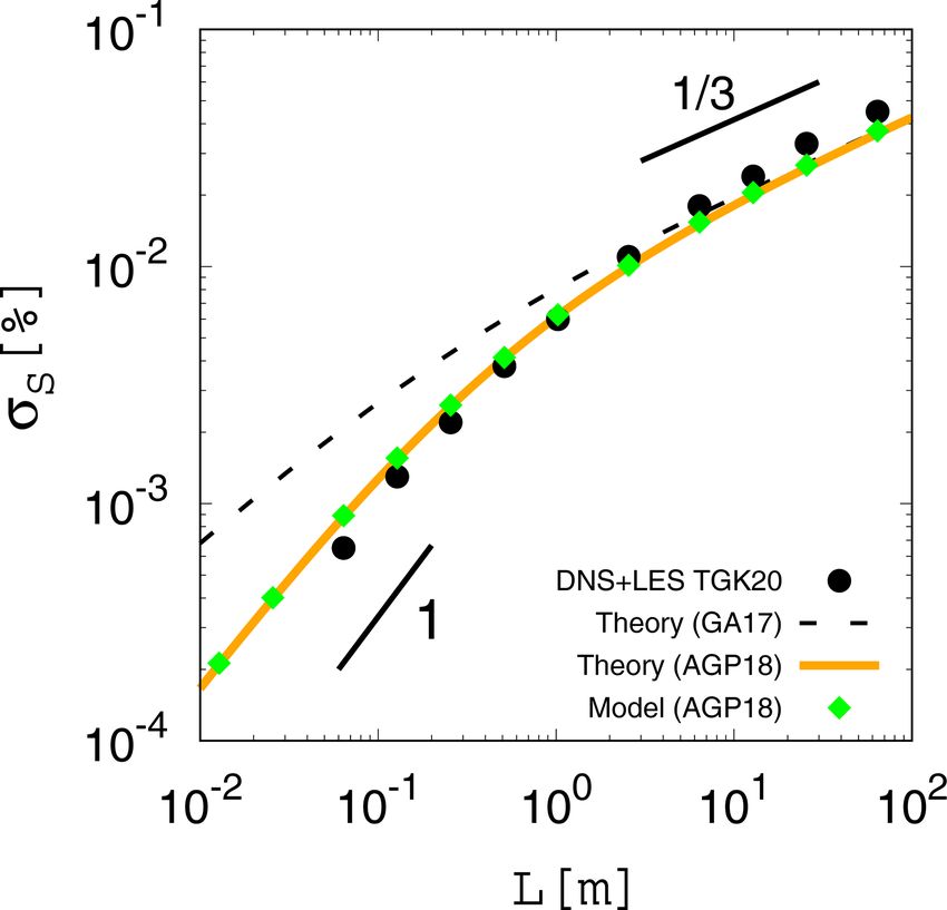
13120                                                I. Saito et al.: Statistical properties of a stochastic model of eddy hopping

data, while the second version successfully reproduces the            two-time covariance defined by
proper scaling. We show how the relaxation term introduced                                      !
by Abade et al. (2018) leads to this improvement. We also                                2σw2 0
                                                                      hFw0 (t)Fw0 (s)i =          δ(t − s),                        (4)
discuss the possibility of simplification of the model, which                              τ
reduces the number of model variables while keeping the sta-
tistical properties almost unchanged in the typical parameter         where the angle brackets indicate an ensemble average and
range for the model implementation in the LES Lagrangian              δ( ) is the Dirac delta function. In the following theoretical
cloud model.                                                          analysis, Eqs. (3) and (2) are used as the governing equations
   The remainder of the present paper is organized as follows.        of the original version.
Section 2 describes the governing equations of the original
version. Section 3 presents a theoretical analysis and numeri-
cal experiments and demonstrates the improper scaling in the          3   Statistical properties of the original version
model prediction by the original version. Section 4 describes
                                                                      We now obtain the analytical expression for the standard de-
the second version. Finally, Sect. 5 discusses the possibility
                                                                      viation of the supersaturation fluctuation, σS 0 , in a statisti-
of simplification of the model.
                                                                      cally steady state. Starting from Eqs. (3) and (2), the result is
                                                                      provided in Eq. (13).
2   Governing equations                                                   First, multiplying Eq. (3) by S 0 and taking an ensemble
                                                                      average, we obtain
The original version of the eddy-hopping model proposed by                     0
                                                                          0 dw          1
Grabowski and Abade (2017) consists of the following two                S          = − hw0 S 0 i                                   (5)
evolution equations. First, the fluctuation of the vertical ve-              dt        τ
locity of turbulent flow at the droplet position, w0 (t), is mod-
                                                                      because of statistical independence hS 0 Fw0 i = 0 . Second,

eled by the Ornstein–Uhlenbeck process:
                                                                      multiplying Eq. (2) by w 0 and taking an ensemble average,
                              q
                                       2δt
                                                                      we obtain
  0             0     −δt/τ
w (t + δt) = w (t)e         + 1 − e− τ σw0 ψ,                 (1)              0
                                                                           0 dS            2       1
                                                                        w          = a1 hw0 i −         hw 0 S 0 i.                (6)
where δt is the time increment, ψ is a Gaussian random num-                  dt                  τrelax
ber with zero mean and unit variance drawn every time step,
                                                                      Summing Eqs. (5) and (6), we obtain
σw0 is the standard deviation of w0 , and τ is the integral time,
or the large-eddy turnover time of the turbulent flow. Here,          d 0 0             2      1                1
σw0 and τ are used as the model parameters. Second, the su-              hw S i = a1 hw0 i −        hw 0 S 0 i − hw0 S 0 i.        (7)
                                                                      dt                     τrelax             τ
persaturation fluctuation at the droplet position, S 0 (t), is gov-
erned by                                                              Next, we consider a statistically steady state. Since
                                                                      an ensemble-averaged variable does not change in time
dS 0              S0                                                  (d h◦i /dt = 0) and hw0 2 i = σw2 0 in the statistically steady
     = a1 w 0 −        .                                       (2)
dt              τrelax                                                state, we obtain the flux of the supersaturation in the verti-
                                                                      cal direction as follows:
Here, the first term on the right-hand side represents the ef-                                 −1
fect of adiabatic cooling and warming due to air parcel as-                            1    1
                                                                      hw0 S 0 i = a1     +          σw2 0
cent and descent caused by the vertical velocity w 0 (t). The                          τ τrelax
parameter a1 has the unit of a scalar gradient. The second                    = a1 (1 + Da)−1 τ σw2 0 ,                            (8)
term on the right-hand side represents the effect of conden-
sation or evaporation of droplets. The timescale τrelax is re-        where Da is the Damköhler number (Shaw, 2003) defined as
ferred to as the phase relaxation time and is inversely propor-
                                                                                τ
tional to the average of the number density and radius of the         Da =             .                                           (9)
droplets (Politovich and Cooper, 1988; Korolev and Mazin,                     τrelax
2003; Kostinski, 2009; Devenish et al., 2012).                        Next, multiplying Eq. (2) by S 0 and taking an ensemble aver-
   Equation (1) can also be written as the following derivative       age, we obtain
form (Pope, 2000):
                                                                      1 d 02                        1        2
dw0    1                                                                   hS i = a1 hw 0 S 0 i −        hS 0 i.                  (10)
    = − w0 (t) + Fw0 (t).                                      (3)    2 dt                        τrelax
 dt    τ
                                                                      In the statistically steady state, we have
Here, the term Fw0 (t) is statistically independent of S 0 and
                                                                                 2
obeys the Gaussian random process that has zero mean and              σS20 = hS 0 i = a1 τrelax hw0 S 0 i.                        (11)

Atmos. Chem. Phys., 21, 13119–13130, 2021                                                  https://doi.org/10.5194/acp-21-13119-2021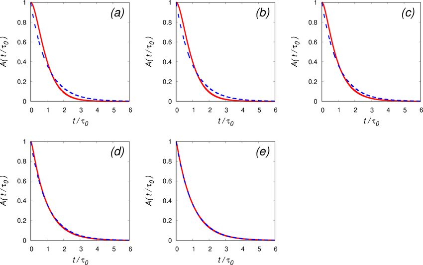
I. Saito et al.: Statistical properties of a stochastic model of eddy hopping                                                      13121

Combining Eqs. (8) and (11), we obtain
                h                      i
σS20 = a1 τrelax a1 (1 + Da)−1 τ σw2 0
   = a12 (1 + Da)−1 τrelax τ σw2 0 ,                         (12)

or equivalently,

σS 0 = (1 + Da)−1/2 Da −1/2 a1 τ σw0 .                       (13)

   Here, σS 0 in Eq. (13) has two important asymptotic forms,
as shown below:
  1. Large scale limit.
     For τ → ∞ (or equivalently, Da → ∞, L → ∞, where
     L = σw0 τ is the integral scale), σS 0 in Eq. (13) is approx-
     imated as                                                       Figure 1. Standard deviation of the supersaturation fluctuation σS 0
                                                                     in the statistically steady state obtained from the analytical expres-
                             1/2
     σS 0 ≈ a1 Da −1/2 τrelax τ 1/2 σw0                              sion given by Eq. (13) (orange curve) and the results of our numeri-
                                                                     cal integration of the original version of the eddy-hopping model
         = a1 τrelax σw0 .                                   (14)
                                                                     (blue squares). The horizontal axis is the integral length L. The
     For the case of a constant dissipation rate of turbulent        black dots indicate the reference data taken from direct numerical
                                                                     simulations and large-eddy simulations by Thomas et al. (2020).
     kinetic energy ε, σw0 ∼ L1/3 (see Appendix B), and we
                                                                     The red triangles indicate the results of the numerical integration of
     have the following scaling:                                     the original version reported by Thomas et al. (2020). The range of
                                                                     L and σS 0 for the panel is the same as in Fig. 10 in Thomas et al.
     σS 0 ∼ L1/3 .                                           (15)
                                                                     (2020). The three short black lines indicate slopes of 1, 2/3, and
                                                                     1/3.
  2. Small scale limit.
     For τ → 0 (or equivalently, Da → 0, L → 0), σS 0 in
     Eq. (13) is approximated as                                     with the theoretical curve (compare the orange curve and the
                 1/2
                                                                     blue squares). As expected based on the analysis, the theoret-
     σS 0 ≈ a1 τrelax τ 1/2 σw0 .                            (16)    ical curve shows the scaling σS 0 ∼ L1/3 for large scales (ap-
                                                                     proximately L > 101 m) and the improper scaling σS 0 ∼ L2/3
     For the case of a constant dissipation rate of turbu-           for small scales (approximately L < 10−1 m). These results
     lent kinetic energy ε, σw0 ∼ L1/3 and τ ∼ L2/3 (see Ap-         are contrary to the results of DNSs and LESs (scaled-up
     pendix B), and we have the following scaling:                   DNSs) conducted by Thomas et al. (2020) (black dots in
     σS 0 ∼ L2/3 .                                           (17)    Fig. 1), which show the proper scalings both for large and
                                                                     small scales (σS 0 ∼ L1/3 and ∼ L1 , respectively).
                                                                        Note that Fig. 1 also shows the results of the numerical
The above asymptotic forms of σS 0 in the two limits can be
                                                                     integration of the original version reported by Thomas et al.
validated through comparison with the result of the scaling
                                                                     (2020) (red triangles), and their results disagree with the re-
argument by Lanotte et al. (2009). From their argument, we
                                                                     sults of the present study. A possible reason for this discrep-
should have σS 0 ∼ a1 τrelax σw0 for the large scale limit, which
                                                                     ancy might be that their results did not achieve a statistically
is consistent with Eq. (14). On the other hand, we should
                                                                     steady state. For details, see Appendix C.
have σS 0 ∼ a1 τ σw0 for the small scale limit, which is incon-
                                                                        The original version of the eddy-hopping model given
sistent with Eq. (16). Therefore, the original version given by
                                                                     by Eqs. (1) and (2) shows the improper scaling for small
Eqs. (3) and (2) does not reproduce the proper scaling for the
                                                                     scales because of the assumption made in the formulation
small scale limit.
                                                                     of the model. Originally, Eq. (2) (corresponding to Eq. 8 in
   Figure 1 compares the scale dependence of σS 0 for the an-
                                                                     Grabowski and Abade, 2017) was formulated under the as-
alytical expression given by Eq. (13) (orange curve) with the
                                                                     sumption of large scales (or Da  1), since this assumption
results of the numerical integration of the original version
                                                                     usually holds for typical situations in atmospheric clouds.
given by Eqs. (1) and (2) (blue squares). Here, numerical in-
                                                                     Thus, it is reasonable that the original version does not re-
tegration is conducted in the same manner as that by Thomas
                                                                     produce the proper scaling for small scales.
et al. (2020) (Sect. 5 of their study), except that the integra-
tion time is increased from 6τ to 10τ (see Appendix A for
details). After the integration time of 10τ , all of the experi-
mental results achieved a statistically steady state and agreed

https://doi.org/10.5194/acp-21-13119-2021                                            Atmos. Chem. Phys., 21, 13119–13130, 2021
13122                                                            I. Saito et al.: Statistical properties of a stochastic model of eddy hopping

4      Statistical properties of the second version                              Finally, the analytical expression corresponding to Eq. (13)
                                                                                 is
We next consider the second version of the eddy-hopping
model by Abade et al. (2018), which is written as follows:                       σS 0 = [1 + (c1 /c2 )Da]−1/2 [2 + (c1 /c2 )Da]−1/2 c1 a1 τ σw0 . (22)
                              q
                                                − (c2δtτ )                         Asymptotic forms of σS 0 in Eq. (22) for the large and small
w0 (t + δt) = w 0 (t)e−δt/(c1 τ ) + 1 − e            1       σw0 ψ,     (18)     scale limits are, respectively, given as follows:
         dS 0                S0         S0
              = a1 w 0 −             −        .                         (19)       1. Large scale limit.
         dt              (c2 τrelax ) (c1 τ )
                                                                                      For τ → ∞ (or equivalently, Da → ∞, L → ∞), σS 0
Note that, for subsequent use, we write the governing equa-                           in Eq. (22) is approximated as
tions in a slightly generalized form by introducing two pa-
rameters c1 and c2 . The second version by Abade et al.                               σS 0 ≈ c2 a1 Da −1 τ σw0
(2018) has c1 = c2 = 1.                                                                   = c2 a1 τrelax σw0 .                                   (23)
   The important change introduced by Abade et al. (2018)
into the original version is the term proportional to −S 0 /τ in                      For the case of a constant dissipation rate of turbulent
Eq. (19). Physically, this term represents the damping effect                         kinetic energy ε, we have
on S 0 due to turbulent mixing (eddy diffusivity). This type
of term is commonly included in stochastic models used in                             σS 0 ∼ L1/3 .                                              (24)
cloud turbulence research (Sardina et al., 2015, 2018; Chan-
drakar et al., 2016; Siewert et al., 2017; Saito et al., 2019a).                   2. Small scale limit.
The timescale of the damping effect due to turbulent mixing                           For τ → 0 (or equivalently, Da → 0, L → 0), σS 0 in
is characterized by the integral time τ , whereas that due to                         Eq. (22) is approximated as
condensation or evaporation of cloud droplets is character-
ized by the phase relaxation time τrelax . The relative impor-                        σS 0 ≈ 2−1/2 c1 a1 τ σw0 ,                                 (25)
tance of these two effects is characterized by the Damköh-                                                         1/2
                                                                                      which indicates that τrelax in Eq. (16) has been replaced
ler number (Da = τ/τrelax ), where the damping effect due to
                                                                                      by τ 1/2 by introducing the term −S 0 /τ in Eq. (19). For
turbulent mixing is dominant for Da  1 (corresponding to
                                                                                      the case of a constant dissipation rate of turbulent ki-
small scales). Below we show that the term −S 0 /τ plays an
                                                                                      netic energy ε, we have
essential role in reproducing the proper scaling.
   Note that it is possible to further extend the second version                      σS 0 ∼ L.                                                  (26)
by additionally introducing the Wiener process term repre-
senting small-scale fluctuations or mixing into Eq. (19) for
                                                                                 Therefore, the second version successfully reproduces
the supersaturation fluctuation. Readers are referred to Paoli
                                                                                 asymptotic forms σS 0 ∼ a1 τrelax σw0 and ∼ a1 τ σw0 for the
and Shariff (2009) and Sardina et al. (2015) for the Langevin
                                                                                 large and small scale limits, respectively, which are both con-
model including such terms, and also to Chandrakar et al.
                                                                                 sistent with the result of the scaling argument by Lanotte
(2021), who implemented such a Langevin model into the
                                                                                 et al. (2009).
LES Lagrangian cloud model and investigated the impact of
                                                                                    Figure 2 (orange curve) shows the theoretical curve given
entrainment mixing and turbulent fluctuations on droplet size
                                                                                 by Eq. (22) for the second version (c1 = c2 = 1). The sec-
distributions in a cumulus cloud. In the present study, how-
                                                                                 ond version reproduces the proper scalings both for large and
ever, we focus on statistical properties of the second version
                                                                                 small scales (σS 0 ∼ L1/3 and ∼ L1 , respectively) and demon-
with Eqs. (18) and (19).
                                                                                 strates better agreement with the reference data (black dots)
   Applying the analytical procedure described in Sect. 3 to
                                                                                 than the original version for L < 100 m. Figure 2 (green di-
the second version given by Eqs. (18) and (19), we first ob-
                                                                                 amonds) also shows the results of the numerical integration
tain
                                                                                 of the second version, which agree with the theoretical curve
                               −1                                              (orange curve), as expected. Here, the numerical integration
                 2        1
   0 0
hw S i = a1         +               σw2 0                                        was conducted in the same manner as in the previous section
                c1 τ c2 τrelax
                                                                                 (see Appendix A for details).
          = c1 a1 [2 + (c1 /c2 )Da]−1 τ σw2 0 ,                         (20)        Although improved, the second version still slightly over-
                                                                                 and underestimates the supersaturation fluctuations for L <
instead of Eq. (8). Next, instead of Eq. (11), we have
                                                                                 3 × 10⁻¹ and L > 2 × 100 m, respectively, as shown in Fig. 2
                                         −1                                    (compare the orange curve with black dots). This deviation
           02             1       1
σS20   = hS i = a1           +                  hw0 S 0 i                        from the reference data can be further reduced by adjusting
                         c1 τ c2 τrelax                                          two parameters c1 and c2 in Eqs. (18) and (19). The analyt-
                = c1 a1 [1 + (c1 /c2 )Da]−1 τ hw 0 S 0 i.               (21)     ical expression (22) and its asymptotic forms (23) and (25)

Atmos. Chem. Phys., 21, 13119–13130, 2021                                                         https://doi.org/10.5194/acp-21-13119-2021
I. Saito et al.: Statistical properties of a stochastic model of eddy hopping                                                      13123

                                                                         c2 has been demonstrated in a recent study on turbulence
                                                                         modulation by particles (Saito et al., 2019b).
                                                                            Here, we do not consider any physical meaning for c1
                                                                         and c2 and use them just as tuning parameters. Two param-
                                                                         eters c1 and c2 are determined by comparing the theoretical
                                                                         curve given by Eq. (22) with the reference data taken from
                                                                         DNSs and LESs in Thomas et al. (2020). The best fit is given
                                                                         by c1 = 0.746 and c2 = 1.28. Figure 3 (solid curve) shows
                                                                         the theoretical curve given by Eq. (22) with these values of
                                                                         c1 and c2 , which agrees almost perfectly with the reference
                                                                         data (black dots). Although the improvement from the sec-
                                                                         ond version with c1 = c2 = 1 is slight, this result shows that
                                                                         the eddy-hopping model can be easily tuned to reproduce the
                                                                         reference data almost perfectly.
Figure 2. Standard deviation of the supersaturation fluctuation σS 0
in the statistically steady state obtained from the analytical expres-   5   Possibility of simplification of the model
sion given by Eq. (22) for the second version (c1 = c2 = 1, orange
curve) and the results of our numerical integration using the second     Finally, we discuss the possibility of simplification of the
version given by Eqs. (18) and (19) (c1 = c2 = 1, green diamonds).       eddy-hopping model. Here, our discussion is based on the
The dashed line indicates the analytical expression given by Eq. (13)    second version given by Eqs. (18) and (19), but the same ar-
for the original version. The two short black lines indicate slopes of   gument also applies to the original version given by Eqs. (1)
1 and 1/3. The black dots and the axes of the panel are the same as
                                                                         and (2).
in Fig. 1.
                                                                            The eddy-hopping model consists of two evolution equa-
                                                                         tions for the supersaturation and vertical velocity fluctua-
                                                                         tions, S 0 and w 0 respectively, and these two variables fluctu-
                                                                         ate randomly according to the Ornstein–Uhlenbeck process.
                                                                         However, if we have S 0 that fluctuates with a proper am-
                                                                         plitude and auto-correlation function, then we do not need
                                                                         the evolution equation for w0 , because only S 0 is used in the
                                                                         growth equation of the droplet size. As described in Sect. 4,
                                                                         we obtained an analytical expression for σS 0 , i.e., the stan-
                                                                         dard deviation of the supersaturation fluctuation in the statis-
                                                                         tically steady state given by Eq. (22). On the other hand, the
                                                                         auto-correlation function for S 0 in a statistically steady state
                                                                         can also be obtained analytically. The derivation is described
                                                                         in Appendix D. The result is given in Eq. (D14) and is as
                                                                         follows:
                                                                                 S 0 (t + t0 )S 0 (t0 )
                                                                         A(t) =                                                      (27)
Figure 3. Standard deviation of the supersaturation fluctuation σS 0              hS 0 (t0 )S 0 (t0 )i
in the statistically steady state from the analytical expression (22)
                                                                                       τ1

                                                                                                               τ2

for the second version. The dashed curve is for c1 = c2 = 1, and the          =                  e−t/τ1 −             e−t/τ2 ,       (28)
solid curve is for c1 = 0.746 and c2 = 1.28. The black dots and the               τ1 − τ2                   τ1 − τ2
axes of the panel are the same as in Fig. 1.                             where τ1 and τ2 are, respectively, defined as
                                                                                                             −1
                                                                                                1        1
                                                                         τ1 = c1 τ, and τ2 =         +
show how c1 and c2 work. These types of parameters are not                                     c1 τ c2 τrelax
new. For example, a parameter corresponding to c1 is com-                                    −1
                                                                                        c1
monly used in the Langevin stochastic equation in turbulence                = c1 τ 1 + Da          .                                 (29)
research (Sawford, 1991; Marcq and Naert, 1998). Formally,                              c2
the inverse of c1 is referred to as the drift coefficient, and           We can also obtain the auto-correlation time for S 0 by time
the coefficients for the velocity and scalar equations should            integration of A(t) (see Eq. D16 in Appendix D), which is
be distinguished. However, we treat these coefficients as the            given as
same parameter in Eqs. (18) and (19) for simplicity. On the
other hand, the importance of a parameter corresponding to               τ0 = τ1 + τ2 .                                              (30)

https://doi.org/10.5194/acp-21-13119-2021                                                 Atmos. Chem. Phys., 21, 13119–13130, 2021
13124 I. Saito et al.: Statistical properties of a stochastic model of eddy hopping
Figure 4. Auto-correlation functions in the statistically steady state for the simplified model (B(t) in Eq. 35: blue dashed curve) and the
second version (A(t) in Eq. 28: red solid curve). Here, c1 = c2 = 1. The parameters for each panel are as follows: (a) L = 10−2 m, τ =
0.447 s, τ0 = 0.844 s, Da = 0.127; (b) L = 10−1 m, τ = 2.08 s, τ0 = 3.38 s, Da = 0.591; (c) L = 100 m, τ = 9.63 s, τ0 = 12.2 s, Da = 2.74;
(d) L = 101 m, τ = 44.7 s, τ0 = 48.0 s, Da = 12.7; and (e) L = 102 m, τ = 208 s, τ0 = 211 s, Da = 59.1. The phase relaxation time is fixed
to τrelax = 3.513 s. The horizontal axis is the time t normalized by the auto-correlation time τ0 for each case. The parameter τ is determined
from the integral length L based on the setting for the numerical experiment described in Appendices A and B.
The auto-correlation function A(t) in Eq. (28) and the auto- model given by Eqs. (18) and (19) before the simplification.
correlation time τ0 in Eq. (30), with τ1 and τ2 defined by (29), The auto-correlation function for S 0 in the simplified model
have important asymptotic forms in two limits. First, for the given by Eq. (33) is as follows:
large scale limit (Da → ∞), the asymptotic forms of A(t)
and τ0 are given by S 0 (t + t0 )S 0 (t0 )
B(t) = (34)
−t/(c1 τ )
hS 0 (t0 )S 0 (t0 )i
lim A(t) = e and lim τ0 = c1 τ, (31)
Da→∞ Da→∞ = e−t/τ0 , (35)
respectively. Second, for the small scale limit (Da → 0), the which has the following two asymptotic forms. First, for the
asymptotic forms of A(t) and τ0 are given by large scale limit (Da → ∞),
t
lim A(t) = 1 + e−t/(c1 τ ) and lim B(t) = e−t/(c1 τ ) , (36)
Da→0 (c1 τ ) Da→∞
lim τ0 = 2c1 τ, (32) which agrees with the corresponding asymptotic form given
Da→0
by Eq. (31) for the second version. Second, for the small
respectively. scale limit (Da → 0),
Based on analytical expressions for the fluctuation ampli-
tude and the auto-correlation function for S 0 (Eqs. 22 and lim B(t) = e−t/(2c1 τ ) , (37)
Da→0
30, respectively), a simplified version of the eddy-hopping
model is defined as follows: which disagrees with the corresponding asymptotic form
q given by Eq. (32) for the second version.
− 2δt Figures 4a through e compare the auto-correlation func-
S 0 (t + δt) = S 0 (t)e−δt/τ0 + 1 − e τ0 σS 0 ψ, (33)
tion for the simplified model (B(t) in Eq. 35: blue dashed
where σS 0 and τ0 are given by Eqs. (22) and (30), respec- curve) and that for the second version (A(t) in Eq. 28: red
tively. Note that the simplified model given by Eq. (33) is solid curve) for five cases ranging from Da
1 to Da
1.
a single-equation model, as compared to the two-equation Here, c1 = c2 = 1. Note that the time t is normalized by
Atmos. Chem. Phys., 21, 13119–13130, 2021 https://doi.org/10.5194/acp-21-13119-2021I. Saito et al.: Statistical properties of a stochastic model of eddy hopping 13125
Figure 5. Time evolutions of the supersaturation fluctuations obtained from the numerical integration of the original version (Eqs. 1 and
2, dashed red curve), the second version (Eqs. 18 and 19, dotted blue curve), and the simplified model (Eq. 33, solid green curve). The
parameters for each panel are as follows: (a) L = 10−2 m, τ = 0.447 s, Da = 0.127; (b) L = 100 m, τ = 9.63 s, Da = 2.74; (c) L = 102 m,
τ = 208 s, Da = 59.1. The phase relaxation time is fixed to τrelax = 3.513 s. Results are shown for the time range 0 ≤ (t/τ − 10) ≤ 10 (or
equivalently, 10τ ≤ t ≤ 20τ ), where all cases are already in a statistically steady state. The numerical integration was conducted in the same
manner as described in Appendix A. All results were obtained by using the same random number series.
the auto-correlation time τ0 for each case. Although B(t) large scales (Fig. 5c, L = 102 m), the simplified model and
and A(t) share the same auto-correlation time, B(t) deviates the second version produce almost identical results.
from A(t) for cases with Da of order unity or smaller, as
shown in Fig. 4a through c. On the other hand, for Da
1,
B(t) agrees with A(t) very well, as shown in Fig. 4d and e. 6 Summary and conclusions
The simplified model has the desirable convergence prop-
The purpose of the present paper was to obtain various
erty. The auto-correlation function for the simplified model
statistical properties of the eddy-hopping model, a novel
(B(t) in Eq. 35) converges to that for the second version in
cloud microphysical model, which accounts for the effect of
the large-scale limit (Da → ∞), as shown in Eq. (36). As
the supersaturation fluctuation at unresolved scales on the
confirmed in Figs. 4d and e, the two auto-correlation func-
growth of cloud droplets and on spectral broadening. Two
tions are almost identical for an integral length L greater
versions of the model are considered: the original version
than 10 m (or Da ≥ 10). In the implementation of the eddy-
by Grabowski and Abade (2017) and the second version by
hopping model to the LES Lagrangian cloud model, the in-
Abade et al. (2018). Based on derived statistical properties,
tegral length L is supposed to roughly correspond to the grid
we first showed in Sect. 3 that the original version fails to
size, which is often greater than several meters to several
reproduce a proper scaling for smaller Damköhler numbers
tens of meters. Therefore, the assumption of large scales (or
(corresponding to small scales), resulting in a deviation of the
Da
1) usually holds, in which case the statistical proper-
model prediction from the reference data taken from DNSs
ties of the simplified model are expected to be almost un-
and LESs, as shown in Fig. 1. In Sect. 4, we showed that
changed after the simplification.
the second version successfully reproduces the proper scal-
Figure 5 compares the time evolutions of the supersatura-
ing and agrees better with the reference data than the origi-
tion fluctuations obtained from the numerical integration of
nal version for small scales (L < 100 m in Fig. 2). We also
the original version (dashed red curve), the second version
showed that, by adjusting two parameters c1 and c2 , the sec-
(dotted blue curve), and the simplified model (solid green
ond version can almost perfectly reproduce the reference
curve). Here, the numerical integration was conducted in the
data. In Sect. 5, we discussed the possibility of simplifica-
same manner as described in Appendix A. All results were
tion of the model. The simplified model consists of a sin-
obtained by using the same random number series. The re-
gle stochastic equation for the supersaturation fluctuation, as
sults are shown in the time range 10τ ≤ t ≤ 20τ , where all
in Eq. (33), with amplitude and time parameters given by
cases are already in a statistically steady state.
the corresponding analytical expressions for the model be-
For small scales, the simplified model produces qualita-
fore the simplification. We showed that, for larger Damköhler
tively different trajectories of S 0 from the second version, as
numbers (corresponding to large scales), the auto-correlation
shown in Fig. 5a (L = 10−2 m; compare the solid green and
function of the supersaturation fluctuation for the simplified
dotted blue curves), even though these two models share the
model converges to that for the model before the simplifi-
same fluctuation amplitude σS 0 and the auto-correlation time
cation. This convergence property is desirable because the
τ0 in the statistically steady state. The difference is smaller
assumption of large scales usually holds in the typical pa-
for intermediate scales (Fig. 5b, L = 100 m). For sufficiently
rameter range for the model implementation in the LES La-
grangian cloud model.
https://doi.org/10.5194/acp-21-13119-2021 Atmos. Chem. Phys., 21, 13119–13130, 202113126 I. Saito et al.: Statistical properties of a stochastic model of eddy hopping
Appendix A: Numerical integration of the eddy-hopping
model
The results of the numerical integration of the original ver-
sion (Eqs. 1 and 2) and the second version (Eqs. 18 and 19)
are shown in Figs. 1 (blue squares) and 2 (green diamonds),
respectively. For these experiments, we used the same set-
ting as that in Sect. 5 in Thomas et al. (2020), except that
the integration time was increased from 6τ to 10τ . We set
a1 = 4.753×10⁻⁴ m−1 , ε = 10 cm2 s−3 , and τrelax = 3.513 s,
and the integral time τ as
1 L
τ= . (A1)
(2π )1/3 σw0
Figure B1. Relationship between the integral scale L and the turbu-
As described in Appendix B, for the case of a constant dis-
lent kinetic energy E. The black dots are taken from the reference
sipation rate of turbulent kinetic energy ε, σw0 is given as a data in Thomas et al. (2020). The orange curve indicates the fitting
function of L. We time integrated the governing equations of function E = αε2/3 L2/3 with α = 0.475.
the model using 12 values of L: L = 0.0128, 0.0256, 0.064,
0.128, 0.256, 0.512, 1.024, 2.56, 6.4, 12.8, 25.6, and 64.0 m.
The time step δt is set as 1/1000 of τ , and the integra- Appendix C: Achievement of a statistically steady state
tion time is 10τ . The numerical scheme is the forward Euler
method. The initial condition is such that w0 (0) = σw0 ψ and We confirm that all of the results of the numerical integration
S 0 (0) = 0. Each result in Figs. 1 (blue squares) and 2 (green of the eddy-hopping model in the present study achieved sta-
diamonds) is obtained by averaging the results for 1000 en- tistically steady states. For this purpose, we first derive the
sembles with different seeds of random numbers. analytical expression for the time evolutions of the variance
and covariance of the variables in the model and then com-
pare these analytical expressions with the results of the nu-
merical integration.
Appendix B: Scalings for the case of a constant The governing equations given by Eqs. (3) and (2) can be
dissipation rate of turbulent kinetic energy rewritten in generalized forms as
We consider classical homogeneous isotropic turbulence, in dw 0 1
which energy is mainly injected into the system at large = − w0 (t) + Fw0 (t), (C1)
dt τ1
scales, cascaded to smaller scales by nonlinear interaction,
dS 0 S 0 (t)
and finally dissipated by the molecular viscosity in the small- = a1 w0 (t) − , (C2)
est scales. In a statistically steady state, the dissipation rate of dt τ2
turbulent kinetic energy is defined as ε. If ε is fixed and the where τ1 and τ2 are the relaxation times for w 0 and S 0 , respec-
integral scale L is changed, then the kinetic energy E scales tively, and the forcing term Fw0 (t) satisfies Eq. (4). Evolution
as follows (Thomas et al., 2020): equations for the variance and covariance of the variables are
derived as follows:
E ∼ (Lε)2/3 . (B1) !
dVw0 (t) 2 2σw2 0
= − Vw0 (t) + , (C3)
The black dots in Fig. B1 show the relation between L and E dt τ1 τ1
in the reference data taken from DNSs and LESs by Thomas
dC(t) 1 1
et al. (2020) (Table 2 of their study). In their simulation, = a1 Vw (t) −
0 + C(t), (C4)
the dissipation rate was fixed to ε = 10 cm2 s−3 . The orange dt τ1 τ2
curve in Fig. B1 indicates the function E = αε2/3 L2/3 , where dVS 0 (t) 2
= − VS 0 (t) + 2a1 C(t), (C5)
α is the fitting parameter. The best fit is given by α = 0.475. dt τ2
The root-mean-square turbulent√velocity is calculated as a
function of L by urms = σw0 = (2E/3), and σw0 is used as where Vw0 (t), C(t), and VS 0 (t) are, respectively, defined as
the parameter in the eddy-hopping model. Note that Thomas
Vw0 (t) = w 0 (t)w 0 (t) , (C6)
et al. (2020) used the same type of large-scale forcing as that
used by Kumar et al. (2012), where the integral length L is C(t) = w 0 (t)S 0 (t) , (C7)
0 0
set to be equal to the box length Lbox . VS 0 (t) = S (t)S (t) . (C8)
Atmos. Chem. Phys., 21, 13119–13130, 2021 https://doi.org/10.5194/acp-21-13119-2021I. Saito et al.: Statistical properties of a stochastic model of eddy hopping 13127
For the numerical integration of the eddy-hopping model by Figure C1 compares the analytical expression given by
Thomas et al. (2020), τ1 = τ and τ2 = τrelax . Since the initial Eq. (C14) (cyan dots) with the results of the numerical in-
conditions for w0 (t) and S 0 (t) are set to w0 (0) = σw0 ψ and tegration of the original version given by Eqs. (1) and (2)
S 0 (0) = 0 in Thomas et al. (2020), the corresponding initial (black crosses). The setting for the numerical experiment is
conditions for the variance and covariance are given by the same as that used in Fig. 1, except that the integration
time is 0.6τ in Fig. C1a and 6τ in Fig. C1b. The results of
Vw0 (0) = σw2 0 , (C9) the numerical integration (black crosses) agree well with the
C(0) = 0, (C10) analytical expression (cyan dots), and both approach the the-
VS 0 (0) = 0. (C11) oretical curve for the statistically steady state (orange curve
in each panel) as the integration time increases. Figure C1a
Solving Eqs. (C3) through (C5) with the initial conditions also indicates that the results of the numerical integration of
given by Eqs. (C9) through (C11), we obtain the eddy-hopping model by Thomas et al. (2020) (red trian-
gles) are fairly close to our results at 0.6τ . Thus, it might be
Vw0 (t) = σw2 0 , (C12) possible that the integration time of their numerical exper-
iment was not long enough to achieve a statistically steady
C(t) = a1 σw2 0 τ3 −t/τ3
1−e , (C13)
state.
VS 0 (t) = a12 σw2 0 τ3 τ2 1 − e−2t/τ2
+ 2a12 σw2 0 τ3 τ4 e−t/τ3 − e−2t/τ2 , (C14)
where τ3 and τ4 are, respectively, defined as
τ1 τ2 τ1 τ2
τ3 = , and τ4 = . (C15)
τ1 + τ2 τ2 − τ1
Figure C1. Standard deviation of the supersaturation fluctuation σS 0 at times t = 0.6τ (a) and t = 6τ (b) obtained from the analytical
expression given by Eq. (C14) (cyan dots) and the results of the numerical integration of the original version given by Eqs. (1) and (2) (black
crosses). The orange curve, red triangles, and axes of the panel are the same as in Fig. 1. The two short black lines indicate slopes of 2/3 and
1/3. The setting for the numerical integration is the same as that used in Sect. 3, except that the integration times are 0.6τ and 6τ in (a) and
(b), respectively.
https://doi.org/10.5194/acp-21-13119-2021 Atmos. Chem. Phys., 21, 13119–13130, 202113128 I. Saito et al.: Statistical properties of a stochastic model of eddy hopping
Appendix D: Derivation of auto-correlation function Multiplying Eq. (D8) by S 0 (0) and taking an ensemble aver-
age, we obtain
We derive the analytical expression for the auto-correlation
function of the supersaturation fluctuation S 0 (t) in the eddy- hS 0 (t)S 0 (0)i = hS 0 (0)S 0 (0)ie−t/τ2 + a1 hw0 (0)S 0 (0)i
hopping model. As in Appendix C, we start from the gener- −1
τ2−1 − τ1−1 e−t/τ1 − e−t/τ2 ,
alized form of the eddy-hopping model as follows: (D9)
dw0 1
= − w 0 (t) + Fw0 (t), because of the statistical independence Fw0 (ζ )S 0 (0) = 0 .
(D1)
dt τ1 Next, as in the derivation of Eq. (11), we multiply Eq. (D2)
dS 0 S 0 (t) by S 0 and consider the statistically steady state. We obtain
= a1 w 0 (t) − , (D2)
dt τ2
where τ1 and τ2 are the relaxation times for w 0 and S 0 , re- hS 0 (0)S 0 (0)i = a1 τ2 hw 0 (0)S 0 (0)i. (D10)
spectively, and the forcing term Fw0 (t) satisfies Eq. (4). We
Substituting Eq. (D10) into (D9), we have
consider that the system is in a statistically steady state.
First, multiplying Eq. (D2) by et/τ2 and applying the prod- hS 0 (t)S 0 (0)i = hS 0 (0)S 0 (0)ie−t/τ2
uct rule of differentiation, we obtain
d 0 + hS 0 (0)S 0 (0)iτ2−1 τ2−1
S (t)et/τ2 = a1 w0 (t)et/τ2 .
(D3) −1
dt
−τ1−1 e−t/τ1 − e−t/τ2 .
(D11)
Integrating Eq. (D3) from t = 0 to t, we obtain
Zt Therefore, the auto-correlation function of the supersatura-
S 0 (t) = S 0 (0)e−t/τ2 + a1 w0 (ξ )e(ξ −t)/τ2 dξ. (D4) tion fluctuation S 0 (t) for the eddy-hopping model given by
Eqs. (D1) and (D2) in the statistically steady state is written
0
as follows:
(Note that we chose the integration range [0, t] for simplicity
of notation. Since we consider a statistically steady state, the hS 0 (t)S 0 (0)i
A(t) = (D12)
following discussion is unchanged if the integration range hS 0 (0)S 0 (0)i
is [t0 , t0 + t].) Applying a similar procedure to that above to τ1
= e−t/τ2 + e−t/τ1 − e−t/τ2
(D13)
Eq. (D1) with the integration range t : 0 → ξ , we obtain τ1 − τ2
Zξ τ1 τ2
= e−t/τ1 − e−t/τ2 . (D14)
0
w (ξ ) = w (0)e 0 −ξ/τ1
+ Fw0 (ζ )e(ζ −ξ )/τ1 dζ. (D5) τ1 − τ2 τ1 − τ2
0 The auto-correlation time τ0 is obtained by time-integrating
Substituting Eq. (D5) into (D4) and calculating some of the A(t) as
integrations, we obtain
Z∞
τ 2 − τ22
Zt τ0 = A(t)dt = 1 (D15)
S 0 (t) = S 0 (0)e−t/τ2 + a1 w 0 (0)e−ξ/τ1 τ1 − τ2
0
0 = τ1 + τ2 . (D16)
Zξ
+ Fw0 (ζ )e(ζ −ξ )/τ1 dζ e(ξ −t)/τ2 dξ (D6) For the original version of the eddy-hopping model given by
Eqs. (1) and (2), we have
0
Zt τ1 = τ, and τ2 = τrelax . (D17)
−1
−τ1−1 )ξ
= S (0)e 0 −t/τ2 0
+ a1 w (0)e −t/τ2
e(τ2 dξ
For the second version given by Eqs. (18) and (19), we have
0
Z t Zξ
−1
1 1
ζ /τ1 (τ2−1 −τ1−1 )ξ τ1 = c1 τ, andτ2 = + . (D18)
+ a1 e−t/τ2 Fw0 (ζ )e e dζ dξ (D7) c1 τ c2 τrelax
0 0
−1
0 −t/τ2
+ a1 w0 (0) τ2−1 − τ1−1 e−t/τ1 − e−t/τ2
= S (0)e
Z t Zξ
−1
−τ1−1 )ξ
+ a1 e −t/τ2
Fw0 (ζ )eζ /τ1 e(τ2 dζ dξ. (D8)
0 0
Atmos. Chem. Phys., 21, 13119–13130, 2021 https://doi.org/10.5194/acp-21-13119-2021I. Saito et al.: Statistical properties of a stochastic model of eddy hopping 13129
Code availability. Programs for numerical integration of the eddy- mos. Sci., 36, 470–483, https://doi.org/10.1175/1520-
hopping model are written in Fortran 90 and are available upon re- 0469(1979)0362.0.CO;2, 1979.
quest. Cooper, W. A.: Effects of variable droplet growth histo-
ries on Droplet size distributions. Part I: Theory, J. At-
mos. Sci., 46, 1301–1311, https://doi.org/10.1175/1520-
Data availability. The data in this study are available upon request. 0469(1989)0462.0.CO;2, 1989.
Devenish, B. J., Bartello, P., Brenguier, J.-L., Collins, L. R.,
Grabowski, W. W., IJzermans, R. H. A., Malinowski, S. P.,
Author contributions. IS conducted the numerical simulations and Reeks, M. W., Vassilicos, J. C., Wang, L.-P., and Warhaft, Z.:
data analysis. IS and TW performed the theoretical analyses in Droplet growth in warm turbulent clouds, Q. J. Roy. Meteor.
Sect. 3 and 4. IS and TG performed the theoretical analysis in Soc., 138, 1401–1429, https://doi.org/10.1002/qj.1897, 2012.
Sect. 5. All three of the authors were involved in preparing the Grabowski, W. W. and Abade, G. C.: Broadening of cloud
manuscript. droplet spectra through eddy hopping: Turbulent adia-
batic parcel simulations, J. Atmos. Sci., 74, 1485–1493,
https://doi.org/10.1175/JAS-D-17-0043.1, 2017.
Grabowski, W. W. and Wang, L.-P.: Growth of cloud droplets in
Competing interests. The authors declare that they have no con-
a turbulent environment, Annu. Rev. Fluid Mech., 45, 293–324,
flicts of interest.
https://doi.org/10.1146/annurev-fluid-011212-140750, 2013.
Korolev, A. V. and Mazin, I. P.: Supersaturation of water vapor in
clouds, J. Atmos. Sci., 60, 2957–2974, 2003.
Disclaimer. Publisher’s note: Copernicus Publications remains Kostinski, A. B.: Simple approximations for condensational growth,
neutral with regard to jurisdictional claims in published maps and Environ. Res. Lett., 4, 015005, https://doi.org/10.1088/1748-
institutional affiliations. 9326/4/1/015005, 2009.
Kumar, B., Janetzko, F., Schumacher, J., and Shaw, R. A.: Extreme
responses of a coupled scalar–particle system during turbulent
Acknowledgements. We are grateful to Kei Nakajima for his techni- mixing, New J. Phys., 14, 115020, https://doi.org/10.1088/1367-
cal support. The present study was supported by MEXT KAKENHI 2630/14/11/115020, 2012.
grant nos. 20H00225 and 20H02066, by JSPS KAKENHI grant no. Lanotte, A. S., Seminara, A., and Toschi, F.: Cloud droplet growth
18K03925, by the Naito Foundation, by the HPCI System Research by condensation in homogeneous isotropic turbulence, J. Atmos.
Project (project ID: hp200072, hp210056), by the NIFS Collabora- Sci., 66, 1685–1697, https://doi.org/10.1175/2008JAS2864.1,
tion Research Program (NIFS20KNSS143), by the Japan High Per- 2009.
formance Computing and Networking plus Large-scale Data Ana- Lasher-Trapp, S. G., Copper, W. A., and Blyth, A. M.: Broaden-
lyzing and Information Systems (jh200006, jh210014), and by High ing of droplet size distributions from entrainment and mixing
Performance Computing (HPC 2020, HPC2021) at Nagoya Univer- in a cumulus cloud, Q. J. Roy. Meteor. Soc., 131, 195–220,
sity. https://doi.org/10.1256/qj.03.199, 2005.
Marcq, P. and Naert, A.: A Langevin equation for the energy cas-
cade in fully developed turbulence, Physica D, 124, 368–381,
Review statement. This paper was edited by Markus Petters and re- https://doi.org/10.1016/S0167-2789(98)00237-1, 1998.
viewed by three anonymous referees. Paoli, R. and Shariff, K.: Turbulent condensation of droplets: Direct
simulation and a stochastic model, J. Atmos. Sci., 66, 723–740,
https://doi.org/10.1175/2008JAS2734.1, 2009.
Politovich, M. K. and Cooper, W. A.: Variability of
References the supersaturation in cumulus clouds, J. Atmos.
Sci., 45, 2064–2086, https://doi.org/10.1175/1520-
Abade, G. C., Grabowski, W. W., and Pawlowska, H.: Broaden- 0469(1988)0452.0.CO;2, 1988.
ing of cloud droplet spectra through eddy hopping: Turbulent Pope, S. B.: Turbulent flows, Cambridge University Press, Cam-
entraining parcel simulations, J. Atmos. Sci., 75, 3365–3379, bridge, 2000.
https://doi.org/10.1175/JAS-D-18-0078.1, 2018. Saito, I., Gotoh, T., and Watanabe, T.: Broadening of cloud droplet
Chandrakar, K. K., Cantrell, W., Chang, K., Ciochetto, D., Nieder- size distributions by condensation in turbulence, J. Meteor.
meier, D., Ovchinnikov, M., Shaw, R. A., and Yang, F.: Aerosol Soc. Japan, 97, 867–891, https://doi.org/10.2151/jmsj.2019-049,
indirect effect from turbulence-induced broadening of cloud- 2019a.
droplet size distributions, P. Natl. Acad. Sci. USA, 113, 14243– Saito, I., Watanabe, T., and Gotoh, T.: A new time scale for
14248, https://doi.org/10.1073/pnas.1612686113, 2016. turbulence modulation by particles, J. Fluid Mech., 880, R6,
Chandrakar, K. K., Grabowski, W. W., Morrison, H., and Bryan, https://doi.org/10.1017/jfm.2019.775, 2019b.
G. H.: Impact of entrainment–mixing and turbulent fluctuations Sardina, G., Picano, F., Brandt, L., and Caballero, R.: Con-
on droplet size distributions in a cumulus cloud: An investigation tinuous growth of droplet size variance due to conden-
using Lagrangian microphysics with a sub–grid–scale model, J. sation in turbulent clouds, Phys. Rev. Lett., 115, 1–5,
Atmos. Sci., https://doi.org/10.1175/JAS-D-20-0281.1, 2021. https://doi.org/10.1103/PhysRevLett.115.184501, 2015.
Clark, T. L. and Hall, W. D.: A numerical exper-
iment on stochastic condensation theory, J. At-
https://doi.org/10.5194/acp-21-13119-2021 Atmos. Chem. Phys., 21, 13119–13130, 202113130 I. Saito et al.: Statistical properties of a stochastic model of eddy hopping
Sardina, G., Picano, F., Brandt, L., and Caballero, R.: Broadening Shaw, R. A.: Particle-turbulence interactions in atmo-
of cloud droplet size spectra by stochastic condensation: effects spheric clouds, Annu. Rev. Fluid Mech., 35, 183–227,
of mean updraft velocity and CCN activation, J. Atmos. Sci., 75, https://doi.org/10.1146/annurev.fluid.35.101101.161125, 2003.
451–467, https://doi.org/10.1175/JAS-D-17-0241.1, 2018. Siewert, R., Bec, J., and Krstulvic, G.: Statistical steady state in
Sawford, B. L.: Reynolds number effects in Lagrangian stochastic turbulent droplet condensation, J. Fluid Mech., 810, 254–280,
models of turbulent dispersion, Phys. Fluids A-Fluid, 3, 1577– https://doi.org/10.1017/jfm.2016.712, 2017.
1586, https://doi.org/10.1063/1.857937, 1991. Thomas, L., Grabowski, W. W., and Kumar, B.: Diffusional growth
Sedunov, Y. S.: Physics of Drop Formation in the Atmosphere, John of cloud droplets in homogeneous isotropic turbulence: DNS,
Wiley and Sons, New York, 1974. scaled-up DNS, and stochastic model, Atmos. Chem. Phys., 20,
9087–9100, https://doi.org/10.5194/acp-20-9087-2020, 2020.
Atmos. Chem. Phys., 21, 13119–13130, 2021 https://doi.org/10.5194/acp-21-13119-2021You can also read