Maximizing the capture velocity of molecular magneto-optical traps with Bayesian optimization - arXiv.org
←
→
Page content transcription
If your browser does not render page correctly, please read the page content below
Maximizing the capture velocity of molecular
                                                   magneto-optical traps with Bayesian optimization
arXiv:2104.07984v1 [physics.atom-ph] 16 Apr 2021

                                                   Supeng Xu, P Kaebert, M Stepanova, T Poll, M Siercke1 , and S Ospelkaus1
                                                   Institut für Quantenoptik, Leibniz Universität Hannover, 30167 Hannover, Germany
                                                   1
                                                     To whom any correspondence should be addressed
                                                   Email: siercke@iqo.uni-hannover.de and silke.ospelkaus@iqo.uni-hannover.de

                                                                Abstract. Magneto-optical trapping (MOT) is a key technique on the route towards
                                                                ultracold molecular ensembles. However, the realization and optimization of magneto-
                                                                optical traps with their wide parameter space is particularly difficult. Here, we present
                                                                a very general method for the optimization of molecular magneto-optical trap operation
                                                                by means of Bayesian optimization (BO). As an example for a possible application,
                                                                we consider the optimization of a calcium fluoride (CaF) MOT for maximum capture
                                                                velocity. We find that both the X 2 Σ+ to A2 Π1/2 and the X 2 Σ+ to B 2 Σ+ transition to
                                                                allow for capture velocities larger than 20 m/s with 24 m/s and 23 m/s respectively
                                                                at a total laser power of 200 mW. In our simulation, the optimized capture velocity
                                                                depends logarithmically on the beam power within the simulated power range of 25
                                                                to 400 mW. Applied to heavy molecules such as BaH and BaF with their low capture
                                                                velocity MOTs it might offer a route to far more robust magneto-optical trapping.
Maximizing the capture velocity of molecular magneto-optical traps with Bayesian optimization2

1. Introduction

Cooling molecules to temperatures near absolute zero is expected to open many exciting
research opportunities ranging from dipolar quantum many-body physics [1] to precision
tests of fundamental physics [2, 3, 4]. Direct laser cooling and trapping [5], which is the
workhorse of cold atom physics, have already been successfully developed for molecules.
While tremendous progress has been achieved in laser cooling of molecules [6, 7, 8],
magneto-optical trapping [9, 10, 11, 12], and conservative trapping using magnetic
[13, 14] and optical [15] traps, the number of molecules loaded from the molecular beam
is currently still limited to about 105 [11, 16]. The biggest limiting factors are the low
efficiency of current slowing methods [17, 18] along with the generally lower flux beam
source [19, 20]. Some methods have been proposed to increase the number of slowed
molecules, such as the Zeeman–Sisyphus decelerator [21] and the molecular Zeeman
slower [22, 23], or to increase the loading efficiency using the stimulated emission force
[24] , but this increase in efficiency still remains to be proven experimentally.
      Zeeman slowing combines the advantages of white light slowing and chirped-light
slowing as it is a continuous method and provides molecules with a well-defined final
velocity [25]. However, after passing the slowing region, the molecules will have a
period of free flight before they reach the center of the trap. This can be problematic
for MOTs that have low capture velocities and rely on a maxed-out slowing region.
Since the remaining transverse velocity of the molecules will result in the expansion of
the molecular cloud, a low longitudinal velocity at the end of the slower means a longer
time of flight, and a larger molecular cloud reaching the trap center. Transverse cooling
of the molecular beam ahead of the slowing process can have an effect on increasing
the number of loaded molecules, but the improvement is limited [26], since the initial
collimated beam will finally expand again due to the directional absorption and random
re-emission of photons [27]. In contrast, an improvement to the capture velocity of the
MOT will increase the MOT population by orders of magnitude [28], which is what we
are seeking to do in this manuscript.
      Previous theoretical studies of molecular MOTs always kept a common detuning
of each laser component to its respective transition, evenly distributed laser intensity
among each laser component, and fixed magnetic gradient and beam diameter [29, 30, 31]
to search for the optimal laser polarization configuration. This is reasonable since it is
hard to select the optimal configurations from such a high-dimensional parameter space.
      In this paper, we use Bayesian optimization [32] together with a rate equation
model [33] to globally search the total parameter space (detuning, polarization and
intensity of each laser frequency component, separately, combined with 1/e2 beam
radius w and magnetic field gradient A) to find the MOT configurations that have
the largest capture velocity for both the X 2 Σ+ to A2 Π1/2 and X 2 Σ+ to B 2 Σ+ transition.
After initial selection, we comprehensively consider five aspects of the force profile,
including the trap frequency, the damping coefficient, the peak values of both trapping
and cooling acceleration and the capture velocity, to choose the optimal configurations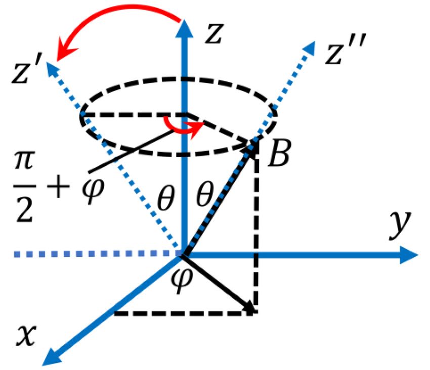
Maximizing the capture velocity of molecular magneto-optical traps with Bayesian optimization3

for the MOT. The optimization tells us that the “dual-frequency” effect is still the main
reason responsible for the force of the X → A DC MOT, but there are experimentally
feasible laser configurations that can provide a better confining and damping force than
the configurations currently used. For the case of the X 2 Σ+ to B 2 Σ+ transition, which
is thought to be not suitable for a MOT because of the large energy splitting of the
upper F = 0 and F = 1 levels [29], we also find some configurations that provide a large
capture velocity and a considerable MOT force. ‡ We investigate the dependence of
capture velocity on the total laser power and find a good linear fit to the logarithm of
laser power from 25 to 400 mW. Our method can be applied to heavy molecules like SrF
[7], BaF [23] and BaH [31] to search for solutions with multiple frequency components
and improve the loading efficiency of the MOT.

2. Rate equation model

We use the rate equation model described in [33] to calculate the force of the CaF
MOT, in which we consider the effect of each laser frequency component from all six
directions. To find the capture velocity for a specific MOT configuration, we place
the molecules at a distance of 20 mm away from the center of the MOT in the z = 0
plane, traveling along the √12 (~x + ~y ) direction with a range of speeds (see Fig. 1). The
location of the molecule is used to determine the magnetic field according to the formula:
B~ = A(~x + ~y − 2~z), which defines the direction of the quantization axis (QA). Then, we
use a rotation matrix to project the effect of any laser polarization on the QA direction
to get the real transition ratio in (σ + , σ − , π). For details, see Appendix A. The velocities
along each axis are used to get the Doppler shift. The validity of our code is verified by
reproducing the results in [29].
     As is shown in Fig. 2, for the X 2 Σ+ to A2 Π1/2 transition, both X 2 Σ+ (v = 0) to
A Π1/2 (v = 0) and X 2 Σ+ (v = 1) to A2 Π1/2 (v = 0) vibrational transitions are considered
  2

to correctly model the excited state populations, while for the X 2 Σ+ to B 2 Σ+ transition,
since the ground v = 0 state and the v = 1 state do not share the same excited state
and the Franck-Condon factor of the X 2 Σ+ (v = 0) to B 2 Σ+ (v = 0) transition is nearly
unity, we only consider the main pump laser. We neglect higher vibrational states,
because their effect on the size and shape of the MOT force is too small. Through
the whole simulation, the fully nonlinear Zeeman splittings of X 2 Σ+ (v = 0, 1, N = 1),
A2 Π1/2 (v = 0, J = 1/2), and B 2 Σ+ (v = 0, N = 0) ro-vibrational states are used.
     The ground and excited state hyperfine levels of both X 2 Σ+ → A2 Π1/2 and X 2 Σ+ →
B 2 Σ+ are shown in the lower part of Fig. 2, along with the energy splitting in units
of decay rate Γ. In the following discussion, the F = 1− , 0, 1+ and 2 are labeled as
i = 1, 2, 3, 4, respectively. In the simulation, each level i is addressed by an individual
laser with independent polarization, intensity ratio and detuning, (σi , Ii , δi ). In order
‡ Note that a realistic scheme for a X 2 Σ+ to B 2 Σ+ state MOT would have to consider a leakage to
the A2 Π1/2 state. However, since the order of magnitude of this leakage is not yet known, this effect is
neglected here.
Maximizing the capture velocity of molecular magneto-optical traps with Bayesian optimization4 Figure 1: Diagram of the scheme used to simulate the MOT and the capture velocity. The two crossed and perpendicular red hollow rectangles represent the counter- propagating laser beams in the xy plane, the red filled circle refers to the third laser beam pair counter-propagating along the z axis. Figure 2: CaF MOT transitions used in the simulation. (a) The X 2 Σ+ → A2 Π1/2 transition. Since both v = 0 and v = 1 lasers address the same upper state, both need to be considered in the rate equations. The lower part shows the hyperfine states where the energy splitting between interconnected levels are labeled in units of Γ. (b) The X 2 Σ+ → B 2 Σ+ transition. While re-pumping due to vibrational relaxation is necessary for this configuration, just as was the case in the X 2 Σ+ → A2 Π1/2 transition, the v = 1 state does not need to be considered in the rate equations since it is pumped over a different excited state, thereby having little influence on the final force. The spacings between hyperfine states are labeled in units of the decay rate from the B 2 Σ+ state.
Maximizing the capture velocity of molecular magneto-optical traps with Bayesian optimization5

Table 1: Parameters adjusted by the Bayesian optimization algorithm and their range

                                Variables      Range
                                    σi          σ + /σ −
                                    Ii           [0, 1]
                                    δi       [−10, 10]Γ
                                    A       [5, 30] G/cm
                                    w        [4, 15] mm

to catch any influence originating from off-resonant laser excitation, we consider the
interactions of each laser with all the four hyperfine levels of the ground state. This
approach works quite well for predicting the CaF spectrum in both low and high
magnetic fields [34]. In order to restrict the calculation to reasonable values and to
speed up the process, each parameter is constrained to lie within certain bounds (see
Table 1).
     Note that the detuning is relative to the frequency difference between level i and
the upper F = 1 state. In the simulation the total laser power is fixed and distributed
among the various frequency components according to Ii . If there is a fifth frequency
component, we choose its detuning such that δ5 = 0 when it addresses the i = 2 level,
and allow for δ5 = −15Γ to 15Γ. In conclusion, our model thus ends up with 14 tunable
parameters in the case of 4 frequency components, and 17 in the case of 5, a parameter
space that would be too large to span by simple loop methods.

3. The Bayesian optimization method

Bayesian optimization is a method particularly suited to the problem at hand. The
method requires no knowledge or assumption about the function we are trying to
evaluate, and it is especially efficient at finding global maxima [35, 36]. The method
models the function we are trying to find as a multivariate Gaussian process [37]. The
optimization starts off with a prior distribution, and, using a particular acquisition
function (e.g. which point has the highest chance of being the maximum), it chooses a
point in parameter space to sample. The thereby obtained information is used to update
the prior, generating a posterior distribution with less uncertainty around the parameter
space where the sample was taken. By treating this posterior as the prior of the next
iteration, Bayesian optimization can efficiently sample a parameter space of up to 20
dimensions to find the global maximum. The global nature of the method is ensured,
because areas in parameter space that have not yet been explored carry with them a
large uncertainty, and will therefore eventually have a higher chance of containing a
maximum when compared to areas that have been excessively sampled. On the other
hand, the method tends to quickly converge to the maximum solution, as it chooses to
sample those areas of parameter space that are most likely to contain the maximum.
Maximizing the capture velocity of molecular magneto-optical traps with Bayesian optimization6
Our simulation is based on the bayesopt function of Matlab Statistics and Machine
Learning Toolbox, which internally uses Gaussian process regression to model the
objective function. We use the default acquisition function, ‘expected-improvement-
per-second-plus’ and a parallel mode to improve the calculation speed. As such, even
though we don’t know the exact relationship between the laser parameters and the
capture velocity, we can calculate the force under a specific laser configuration and
simulate a MOT with this force to get the maximum capture velocity. Note that the
bayesopt function always searches for the minimum value. To get the maximum value,
we therefore turn the capture velocity into a negative number in the program.
4. Results
Using Bayesian optimization we try to find the set of parameters giving the maximum
capture velocity of a MOT for both the X 2 Σ+ → A2 Π1/2 and X 2 Σ+ → B 2 Σ+ transition
of CaF. We set a total power of 200 mW for the main pump laser, and distribute it
according to the number and intensity ratio of laser components. In the cases where
there is a re-pump laser, its power is set to be the same as the pump laser but evenly
distributed among the four hyperfine states and the values of detuning are all set to
zero. The polarization of the re-pump laser has little effect on the final result. In this
paper, we therefore set all the polarization from the positive direction to be σ + . We
find both the X 2 Σ+ → A2 Π1/2 and X 2 Σ+ → B 2 Σ+ transition to have nearly the same
maximum capture velocity. We also study the dependence of maximum capture velocity
on laser power and observe a logarithmic dependence of the capture velocity on the laser
power. Additionally, we check whether adding an additional frequency component will
result in an even better MOT operation, but do not find a significant improvement. We
therefore restrict our discussion to the four laser frequency case.
4.1. The X 2 Σ+ to A2 Π1/2 transition
The optimization results for the X 2 Σ+ to A2 Π1/2 transition are shown in Fig. 3. We plot
the capture velocity for each iteration of the code. The red line is the maximum capture
velocity observed as a function of iteration number. Starting from 0 m/s, the maximum
value of 24 m/s is obtained after ∼400 iterations. We continue the calculation until
1000 iterations to check for even better results. It is worth keeping in mind that, while
we will concentrate on the laser configurations for the 24 m/s capture velocities in the
following discussion, configurations with slightly lower velocities may be meaningful to
consider if other factors (such as MOT size or temperature) are more important, because
the program always pursues the maximum capture velocity and ignores the balance of
confining and damping force.
Table 2 lists the set of parameters that can provide capture velocities of 24 m/s.
All the numbers are rounded to one decimal place. For simplicity, we label a specific
set of parameters with scheme index j where j = 1, 2, . . . , 12. We calculate both theMaximizing the capture velocity of molecular magneto-optical traps with Bayesian optimization7
Figure 3: Optimization of the capture velocity of an X 2 Σ+ → A2 Π1/2 MOT with a total
power of 200 mW. The blue circles show the capture velocity for each iteration of the
BO algorithm. The red solid line represents the maximum capture velocity among all
the searched results up to that trial.
Table 2: A group of optimized parameters that can give a maximum capture velocity
of 24 m/s for the X 2 Σ+ → A2 Π1/2 MOT at a power of 200 mW.
acceleration of a molecule at rest as a function of its displacement from the center of
the trap along √12 (~x + ~y ) direction, and the acceleration of a molecule at the center of
the trap versus its speed for all the schemes in table 2. We find scheme 1 and scheme 5
have better performance in terms of cooling and trapping force in addition to capture
velocity and are fairly straightforward to realize experimentally.
The corresponding trapping and cooling acceleration curves are illustrated in
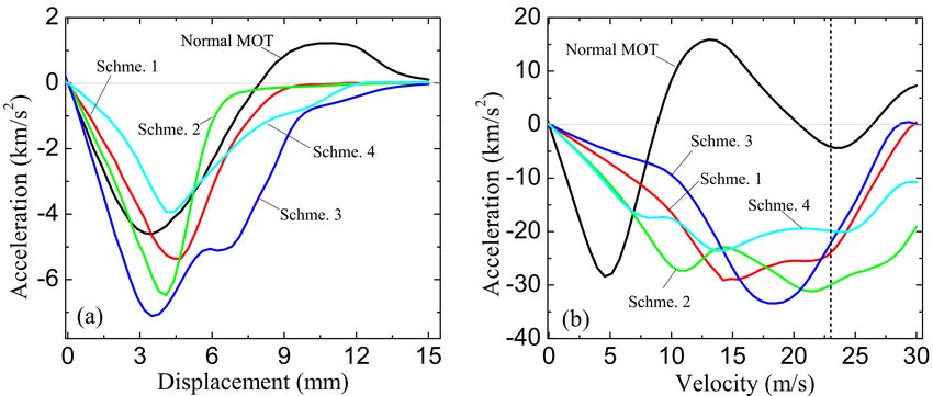
Fig. 4(a) and (b), where we compare the results for scheme 1 and 5 to the results ofMaximizing the capture velocity of molecular magneto-optical traps with Bayesian optimization8 Figure 4: Acceleration versus (a) displacement and (b) velocity, for two of the optimized schemes after comprehensively considering trap frequency, damping coefficient and peak values of both trapping and cooling force. The dashed vertical line reflects the maximum capture velocity, 24 m/s. The acceleration of the currently employed MOT scheme is also plotted for comparison. The laser power is fixed to 200 mW in total. Acceleration versus (c) displacement and (d) velocity, for scheme 5, where I = 1.4% is multiplied by various factors (0, 0.5, 1, 2, 4, 10), keeping the other intensities fixed. Figure 5: Maximum capture velocity versus total laser power for X 2 Σ+ → A2 Π1/2 MOT. The x axis is in logarithmic scale.
Maximizing the capture velocity of molecular magneto-optical traps with Bayesian optimization9

a conventional MOT configuration with evenly distributed laser power among the four
hyperfine states, a common detuning of −Γ, as well as A = 15 G/cm and w = 8 mm.
We see (compare Fig. 4(a) ) that the confining forces for schemes 1 and 5 are similar to
the conventional MOT scheme, while the cooling force is significantly extended towards
larger velocities for the optimized schemes (compare Fig. 4 (b)).
     In scheme 5, it is striking that there is a particular frequency component with a very
low intensity fraction (I3 = 1.4%). It is therefore interesting to investigate whether I3
can be set to zero. The force for various factors of I3 = 1.4 % × n (n = 0, 0.5, 1, 2, 4, 10)
is shown in Fig. 4(c) and (d). Unexpectedly, when n = 0 , we find the peak value of
trapping acceleration is reduced by a factor of 3, while the cooling acceleration has
changed only a little. From n = 0 to n = 4, the trap frequency and the peak trapping
acceleration amplitude keep increasing, and stay strong even up to n = 10. In contrast,
the damping coefficient and the peak cooling acceleration amplitude decrease with the
increase of n. All these characteristics show that the optimization results are stable and
that one can make fine tuning around the optimal configurations to potentially simplify
the experiment.
     Lastly we study the dependence of the maximum capture velocity on the total
power. For each power, we run the BO algorithm and find the optimized maximum
capture velocity. The result is shown in Fig. 5, where the blue circles are simulated
results, and the red solid line is a linear fit (note the log scale of power in the plot).
Each point is the optimized result after 500 trials. From 25 mW to 400 mW, the velocity
changes from 13 m/s to 27 m/s.

4.2. The X 2 Σ+ to B 2 Σ+ transition
The X 2 Σ+ to B 2 Σ+ transition has more favorable Franck-Condon factors, and the re-
pump lasers don’t need to share the same excited states with the pump laser, which
means we can get larger scattering rates while using less power for the re-pumper.
However, the hyperfine splitting of 20 MHz in the upper (B 2 Σ+ ) state has made the
B 2 Σ+ state unsuitable for a MOT with current schemes [29]. While the regular MOT
scheme does not seem to work well, using the BO method we find a maximum capture
velocity of 23 m/s, along with lots of other choices with moderate capture velocities. The
optimization process is shown in Fig. 6, where the circular points are various trials, and
the red solid line is the maximum capture velocity up to that number of iteration. We
found four different sets of configuration that provide the maximum capture velocity
while still being tractable in an experiment. The specific parameters for these four
configurations are listed in Table 3. Some interesting observations can be made from
the data in the table. First, the closest laser component to the i = 4 level is I3 , with a
σ − polarization, while laser I4 , with σ + polarization, mainly addresses the i = 3 level.
This is totally different from the suggested “dual-frequency” arrangement of the X → B
transition MOT [29], where positive and negative polarization laser components address
i = 4 and i = 3 states, separately. Furthermore, the nearest laser component to i = 1
Maximizing the capture velocity of molecular magneto-optical traps with Bayesian optimization10
Figure 6: Optimization of the capture velocity of an X 2 Σ+ → B 2 Σ+ MOT at a power
of 200 mW. The blue circles show the capture velocity for each of the 1000 trials of the
program. The red solid line represents the maximum capture velocity among all the
searched results up to that trial.
level is I2 in scheme 3, which is still > 5Γ detuned from the i = 1 level. This is because
of the energy difference of 3.1Γ in the B state, such that a detuning of −5.1Γ relative
to the upper F = 1 level means a detuning of −2Γ relative to the upper F = 0 state,
and the i = 1 level is mainly coupled to the upper F = 0 state. We also notice that the
small proportion of laser intensity of I4 is necessary for the large confining force.
Table 3: Experimentally feasible groups of optimized parameters that can give a
maximum capture velocity of 23 m/s for the X 2 Σ+ → B 2 Σ+ MOT at a power of 200 mW.
Fig. 7(a) and (b) compare the confining force and the cooling force of the
conventional X 2 Σ+ to B 2 Σ+ MOT scheme [29] to the schemes resulting from the
optimization. First of all, it is important to note that the inversion of the forces observed
in the conventional MOT scheme disappears for the optimized schemes 1 to 4. Unlike
the normal MOT scheme, where the damping acceleration is inverted at 9 m/s, there is
strong cooling force for speeds up to 30 m/s for the four new schemes. All the optimized
schemes have a plateau at large displacement, where the confining force gradually tendsMaximizing the capture velocity of molecular magneto-optical traps with Bayesian optimization11
Figure 7: Acceleration versus (a) displacement and (b) speed, for four optimized sets of
parameters. The acceleration of the MOT scheme in [29] is also plotted for comparison.
The laser power is fixed to 200 mW in total.
Figure 8: Maximum capture velocity versus total laser power for X 2 Σ+ → B 2 Σ+ MOT.
The x axis is in logarithm scale.
to zero. Scheme 3 has the largest peak acceleration of 7120 m/s2 , and the maximum
trap frequency of 243 Hz, but its damping coefficient is quite small as shown in Fig. 7(b).
A compromise of trapping and cooling is scheme 2, where the trap frequency is 198 Hz,
and the damping coefficient is 2022 s−1 . The dashed vertical line in Fig. 7(b) reflects the
maximum capture velocity, 23 m/s.
The maximum capture velocity of X 2 Σ+ → B 2 Σ+ MOT versus the total laser power
is shown in Fig. 8, in which the blue circles are simulated results and the red solid line
is a logarithmic fit to the maximum capture velocity as a function of power. Each data
point is the optimal result after 500 iterations. We plot these results here for guiding
our future experiments in how much laser power is needed to obtain enough captureMaximizing the capture velocity of molecular magneto-optical traps with Bayesian optimization12 velocity. Note that the success of this scheme depends on the exact value of a leakage from the B 2 Σ+ to the A2 Π1/2 state which is currently unknown. Any loss > 10−7 would complicate a B 2 Σ+ -state MOT because the N = 0 and N = 2 states would need to be reintroduced into the cooling cycle. 5. Conclusion In conclusion, we applied the Bayesian optimization approach to search for the maximum capture velocity of a molecular MOT, in which 14 - 17 totally independent parameters are considered. We obtained a group of configurations which can give a capture velocity of 24 m/s for the X 2 Σ+ → A2 Π1/2 transition at 200 mW, along with a large amount of choices with moderate capture velocities. For the X 2 Σ+ to B 2 Σ+ transition, the BO method also gives possible choices with a large capture velocity. We further studied the maximum capture velocity under different values of laser power for both kinds of transition, and find a logarithmic dependency of the capture velocity on laser power. The laser configurations found through this optimization are experimentally feasible and robust with respect to small changes in parameters. We have shown Bayesian optimization to be a great tool in finding parameters that optimize experiments. Other possible uses for the technique is searching for the best trap frequency or damping coefficient after MOT loading, or to investigate molecule capturing with even less laser components. Our approach is completely general and may be used, for example, to investigate possible MOT configurations for the heavier molecules which currently suffer from low capture velocities. Acknowledgement P. K., M. St. and M. S. thank the DFG for financial support through RTG 1991. We gratefully acknowledge financial support through Germany’s Excellence Strategy – EXC-2123/1 QuantumFrontiers.
Maximizing the capture velocity of molecular magneto-optical traps with Bayesian optimization13
Appendix A. Rotation Matrix
We initially define a group of unit polarization matrices within the lab frame,
√ 1 √ 1 0
+ 2 − 2
σ = × −i , σ = × i , Π = 0 , (A.1)
2 2
0 0 1
where z axis is the quantization axis (QA).
Once the magnetic field B is not along the QA direction, we use two-step rotation
to get the polarization matrices of (σ + , σ − , Π) under the local frame, in which B defines
the QA direction, as illustrated in Fig. A1. The first step is rotating about x axis by an
angle θ, in which the matrix is
1 0 0
Rx = 0 cos(θ) − sin(θ) (A.2)
0 sin(θ) cos(θ)
The second step is rotating from z 0 to z 00 around z axis with an angle of π
2
+ϕ
cos( π2 + ϕ) − sin( π2 + ϕ) 0
Rz = sin( π2 + ϕ) cos( π2 + ϕ) 0 (A.3)
0 0 1
Finally, we just project our laser polarization under the lab frame on the three unit
matrices under the local frame to get the real transition ratio in (σ + , σ − , Π).
Figure A1: Diagram of the rotation process, the θ is the angle between the magnetic field
B and the positive z axis, the ϕ is the azimuthal angle. The blue solid arrow defines the
lab frame, the blue dashed arrow reflects the variation of z axis during rotation process
and the red arrow reflects the rotational direction.Maximizing the capture velocity of molecular magneto-optical traps with Bayesian optimization14
References
[1] Yan B, Moses S A, Gadway B, Covey J P, Hazzard K R A, Rey A M, Jin D S and Ye J 2013
Nature 501 521–525 ISSN 1476-4687 URL https://doi.org/10.1038/nature12483
[2] Hudson J J, Kara D M, Smallman I J, Sauer B E, Tarbutt M R and Hinds E A 2011 Nature 473
493–496 ISSN 1476-4687 URL https://doi.org/10.1038/nature10104
[3] Andreev V, Ang D G, DeMille D, Doyle J M, Gabrielse G, Haefner J, Hutzler N R, Lasner
Z, Meisenhelder C, O’Leary B R, Panda C D, West A D, West E P, Wu X and ACME
Collaboration 2018 Nature 562 355–360 ISSN 1476-4687 URL https://doi.org/10.1038/
s41586-018-0599-8
[4] Cairncross W B, Gresh D N, Grau M, Cossel K C, Roussy T S, Ni Y, Zhou Y, Ye J and
Cornell E A 2017 Phys. Rev. Lett. 119(15) 153001 URL https://link.aps.org/doi/10.1103/
PhysRevLett.119.153001
[5] Chu S 1998 Rev. Mod. Phys. 70(3) 685–706 URL https://link.aps.org/doi/10.1103/
RevModPhys.70.685
[6] Lim J, Almond J R, Trigatzis M A, Devlin J A, Fitch N J, Sauer B E, Tarbutt M R and
Hinds E A 2018 Phys. Rev. Lett. 120(12) 123201 URL https://link.aps.org/doi/10.1103/
PhysRevLett.120.123201
[7] Shuman E S, Barry J F and DeMille D 2010 Nature 467 820–823 ISSN 1476-4687 URL
https://doi.org/10.1038/nature09443
[8] Augenbraun B L, Lasner Z D, Frenett A, Sawaoka H, Miller C, Steimle T C and Doyle J M 2020
New Journal of Physics 22 022003 publisher: IOP Publishing URL https://doi.org/10.1088/
1367-2630/ab687b
[9] Truppe S, Williams H J, Hambach M, Caldwell L, Fitch N J, Hinds E A, Sauer B E and Tarbutt
M R 2017 Nature Physics 13 1173–1176 ISSN 1745-2481 URL https://doi.org/10.1038/
nphys4241
[10] Norrgard E B, McCarron D J, Steinecker M H, Tarbutt M R and DeMille D 2016 Phys. Rev. Lett.
116(6) 063004 URL https://link.aps.org/doi/10.1103/PhysRevLett.116.063004
[11] Anderegg L, Augenbraun B L, Chae E, Hemmerling B, Hutzler N R, Ravi A, Collopy A, Ye J,
Ketterle W and Doyle J M 2017 Phys. Rev. Lett. 119(10) 103201 URL https://link.aps.
org/doi/10.1103/PhysRevLett.119.103201
[12] Collopy A L, Ding S, Wu Y, Finneran I A, Anderegg L, Augenbraun B L, Doyle J M and Ye J 2018
Phys. Rev. Lett. 121(21) 213201 URL https://link.aps.org/doi/10.1103/PhysRevLett.
121.213201
[13] Williams H J, Caldwell L, Fitch N J, Truppe S, Rodewald J, Hinds E A, Sauer B E and
Tarbutt M R 2018 Phys. Rev. Lett. 120(16) 163201 URL https://link.aps.org/doi/10.
1103/PhysRevLett.120.163201
[14] McCarron D J, Steinecker M H, Zhu Y and DeMille D 2018 Phys. Rev. Lett. 121(1) 013202 URL
https://link.aps.org/doi/10.1103/PhysRevLett.121.013202
[15] Anderegg L, Cheuk L W, Bao Y, Burchesky S, Ketterle W, Ni K K and Doyle J M 2019
Science 365 1156–1158 ISSN 0036-8075 publisher: American Association for the Advancement
of Science eprint: https://science.sciencemag.org/content/365/6458/1156.full.pdf URL https:
//science.sciencemag.org/content/365/6458/1156
[16] Ding S, Wu Y, Finneran I A, Burau J J and Ye J 2020 Phys. Rev. X 10(2) 021049 URL
https://link.aps.org/doi/10.1103/PhysRevX.10.021049
[17] Truppe S, Williams H J, Fitch N J, Hambach M, Wall T E, Hinds E A, Sauer B E and
Tarbutt M R 2017 New Journal of Physics 19 022001 publisher: IOP Publishing URL
https://doi.org/10.1088/1367-2630/aa5ca2
[18] Barry J F, Shuman E S, Norrgard E B and DeMille D 2012 Phys. Rev. Lett. 108(10) 103002 URL
https://link.aps.org/doi/10.1103/PhysRevLett.108.103002
[19] Barry J F, Shuman E S and DeMille D 2011 Phys. Chem. Chem. Phys. 13 18936–18947 publisher:Maximizing the capture velocity of molecular magneto-optical traps with Bayesian optimization15
The Royal Society of Chemistry URL http://dx.doi.org/10.1039/C1CP20335E
[20] Hutzler N R, Parsons M F, Gurevich Y V, Hess P W, Petrik E, Spaun B, Vutha A C, DeMille
D, Gabrielse G and Doyle J M 2011 Phys. Chem. Chem. Phys. 13 18976–18985 publisher: The
Royal Society of Chemistry URL http://dx.doi.org/10.1039/C1CP20901A
[21] Fitch N J and Tarbutt M R 2016 ChemPhysChem 17 3609–3623 eprint:
https://chemistry-europe.onlinelibrary.wiley.com/doi/pdf/10.1002/cphc.201600656 URL
https://chemistry-europe.onlinelibrary.wiley.com/doi/abs/10.1002/cphc.201600656
[22] Petzold M, Kaebert P, Gersema P, Siercke M and Ospelkaus S 2018 New Journal of Physics 20
042001 publisher: IOP Publishing URL https://doi.org/10.1088/1367-2630/aab9f5
[23] Liang Q, Bu W, Zhang Y, Chen T and Yan B 2019 Phys. Rev. A 100(5) 053402 URL https:
//link.aps.org/doi/10.1103/PhysRevA.100.053402
[24] Wenz K, Kozyryev I, McNally R L, Aldridge L and Zelevinsky T 2020 Phys. Rev. Research 2(4)
043377 URL https://link.aps.org/doi/10.1103/PhysRevResearch.2.043377
[25] Petzold M, Kaebert P, Gersema P, Poll T, Reinhardt N, Siercke M and Ospelkaus S 2018 Phys.
Rev. A 98(6) 063408 URL https://link.aps.org/doi/10.1103/PhysRevA.98.063408
[26] Lunden W, Du L, Cantara M, Barral P, Jamison A O and Ketterle W 2020 Phys. Rev. A 101(6)
063403 URL https://link.aps.org/doi/10.1103/PhysRevA.101.063403
[27] Plotkin-Swing B, Wirth A, Gochnauer D, Rahman T, McAlpine K E and Gupta S 2020 Review
of Scientific Instruments 91 093201 eprint: https://doi.org/10.1063/5.0011361 URL https:
//doi.org/10.1063/5.0011361
[28] Seo B, Chen P, Chen Z, Yuan W, Huang M, Du S and Jo G B 2020 Phys. Rev. A 102(1) 013319
URL https://link.aps.org/doi/10.1103/PhysRevA.102.013319
[29] Tarbutt M R and Steimle T C 2015 Phys. Rev. A 92(5) 053401 URL https://link.aps.org/
doi/10.1103/PhysRevA.92.053401
[30] Xu S, Xia M, Gu R, Yin Y, Xu L, Xia Y and Yin J 2019 Phys. Rev. A 99(3) 033408 URL
https://link.aps.org/doi/10.1103/PhysRevA.99.033408
[31] McNally R L, Kozyryev I, Vazquez-Carson S, Wenz K, Wang T and Zelevinsky T 2020 New Journal
of Physics 22 083047 publisher: IOP Publishing URL https://doi.org/10.1088/1367-2630/
aba3e9
[32] Shahriari B, Swersky K, Wang Z, Adams R P and de Freitas N 2016 Proceedings of the IEEE 104
148–175
[33] Tarbutt M R 2015 New Journal of Physics 17 015007 publisher: IOP Publishing URL https:
//doi.org/10.1088/1367-2630/17/1/015007
[34] Kaebert P and et al 2021 in preparation
[35] Jones D R, Schonlau M and Welch W J 1998 Journal of Global Optimization 13 455–492 ISSN
1573-2916 URL https://doi.org/10.1023/A:1008306431147
[36] Snoek J, Larochelle H and Adams R P 2012 Practical Bayesian Optimization of Machine Learning
Algorithms Advances in Neural Information Processing Systems vol 25 ed Pereira F, Burges
C J C, Bottou L and Weinberger K Q (Curran Associates, Inc.) URL https://proceedings.
neurips.cc/paper/2012/file/05311655a15b75fab86956663e1819cd-Paper.pdf
[37] Rasmussen C E and Williams C K I 2006 Gaussian Processes for Machine Learning (MIT Press)
ISBN 0-262-18253-XYou can also read