Supplementary Online Content
←
→
Page content transcription
If your browser does not render page correctly, please read the page content below
Supplementary Online Content

                Maharana A, Nsoesie EO. Use of deep learning to examine the association of the built
                environment with prevalence of neighborhood adult obesity. JAMA Netw Open.
                2018;1(4):e181535. doi:10.1001/jamanetworkopen.2018.1535

                eMethods. Materials and Data Analysis
                eTable 1. Places of Interest
                eTable 2. Demographic and Obesity Data
                eFigure 1. Illustration of Transfer Learning Approach
                eFigure 2. VGG-CNN-F Convolutional NN Architecture
                eFigure 3. t-SNE Visualization of Features Extracted From VGG-CNN-F for Satellite
                Imagery
                eFigure 4. Actual Obesity Prevalence and Cross-validated Model Estimates of Obesity
                Prevalence
                eFigure 5. Google Satellite Images for Seattle Showing Locations With Low and High
                Obesity Prevalence, Respectively
                eFigure 6. Actual Obesity Prevalence and Cross-validated Model Estimates of Obesity
                Prevalence
                eFigure 7. Google Satellite Images for San Antonio Showing Locations With Low and
                High Obesity Prevalence, Respectively
                eFigure 8. Actual Obesity Prevalence and Cross-validated Model Estimates of Obesity
                Prevalence
                eFigure 9. Google Satellite Images for Memphis Showing Locations With Low and High
                Obesity Prevalence, Respectively
                eFigure 10. Actual Obesity Prevalence and Cross-validated Model Estimates of Obesity
                Prevalence
                eFigure 11. Google Satellite Images for Los Angeles Showing Locations With Low and
                High Obesity Prevalence, Respectively
                eFigure 12. Out-of-Sample Predictions of Obesity Prevalence Plotted Against Actual
                Obesity Prevalence
                eFigure 13. Cross-validated Model Estimates of Per Capita Income Plotted Against
                Actual Per Capita Income
                eFigure 14. Out-of-Sample Model Predictions of Per Capita Income Plotted Against
                Actual Per Capita Income
                eFigure 15. Actual Per Capita Income and Cross-validated Model Estimates of Per
                Capita Income
                eFigure 16. Actual Per Capita Income and Cross-validated Model Estimates of Per
                Capita Income
                eReferences.

                This supplementary material has been provided by the authors to give readers
                additional information about their work.

                                                                  © Maharana A et al. JAMA Network Open.

Downloaded From: https://jamanetwork.com/ on 06/02/2021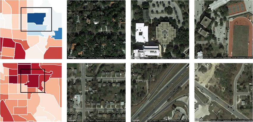
© Maharana A et al. JAMA Network Open.

Downloaded From: https://jamanetwork.com/ on 06/02/2021
eMethods. Materials and Data Analysis

                Data on Obesity Prevalence

                We obtained 2014 estimates on annual crude obesity prevalence from the 500 cities project1. We

                used crude obesity prevalence estimates from 2014 because adjusted estimates and more recent

                annual estimates were unavailable. These obesity estimates are derived from data from the

                United States Centers for Disease Control and Prevention (CDC) Behavioral Risk Factor

                Surveillance System (BRFSS)2. BRFSS is an annual cross-sectional telephone survey used to

                measure behavioral risk factors of U.S. residents. The BRFSS includes all 50 U.S. states, the

                District of Columbia and U.S. territories (i.e., Puerto Rico, Guam and the Virgin Islands).

                An individual is considered obese if their body mass index (BMI) is greater than or equal to 30

                kg/m2, where BMI is estimated from self-reported weight and height. Certain exclusions were

                applied, including removal of pregnant women and individuals reporting certain height and

                weight measurements3. The data includes respondents 18 years of age and older.

                To illustrate our approach, we focused on estimates of obesity prevalence for census tracts in six

                cities – Los Angeles, California; Memphis, Tennessee; San Antonio, Texas; and Seattle, Tacoma

                and Bellevue, Washington. Because Seattle, Tacoma and Bellevue are neighboring cities with

                few census tracts, we combined their data into a single dataset, referred to as, Seattle. These

                cities were selected to reflect regions with varying obesity prevalence. Recent rankings of

                obesity prevalence by states lists Tennessee and Texas as sixth and eighth of fifty most obese

                                                                    © Maharana A et al. JAMA Network Open.

Downloaded From: https://jamanetwork.com/ on 06/02/2021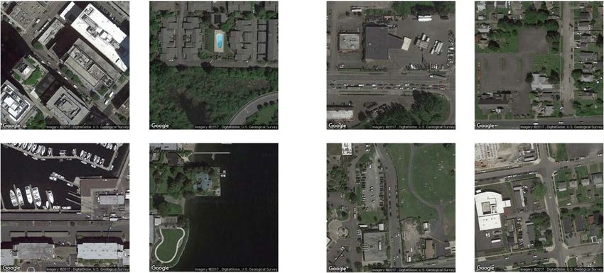
states, respectively4. In contrast, the states of Washington and California have lower obesity rates

                and are ranked thirty-second and forty-seventh of fifty, respectively.

                Satellite Imagery and Places of Interest Data

                We downloaded recent satellite images for each census tract at the zoom level of 18 and image

                dimensions of 400 by 400 pixels (which was later resized to 224 x 224 for our analysis) from the

                freely available Google Static Maps API. Historical data matching the time period of the obesity

                estimates was unavailable. The satellite imagery data consisted of approximately 150,000

                images, implying there were multiple images for each census tract. We also obtained a

                comprehensive list of places of interest (e.g., parks, restaurants, liquor stores, bus stations, night

                clubs) by performing a nearby search for each location in a square grid spanning a census tract,

                using the Google Nearby Search API. We included all categories of places of interest available

                through the API instead of focusing only on physical activity facilities, food and health locations

                which have been widely studied, because we reasoned that other categories could influence an

                individual’s health behavior and physical activity frequency. For example, a high density of pet

                stores could indicate high pet ownership which could influence how often people go to parks and

                take walks around the neighborhood. Furthermore, the places of interest data varied by city, with

                some cities, such as Los Angeles, having finer classifications than others. The data was further

                cleaned to avoid duplicate counts of the same location. A comprehensive list of places of interest

                categories are included in the eTable 1.

                                                                     © Maharana A et al. JAMA Network Open.

Downloaded From: https://jamanetwork.com/ on 06/02/2021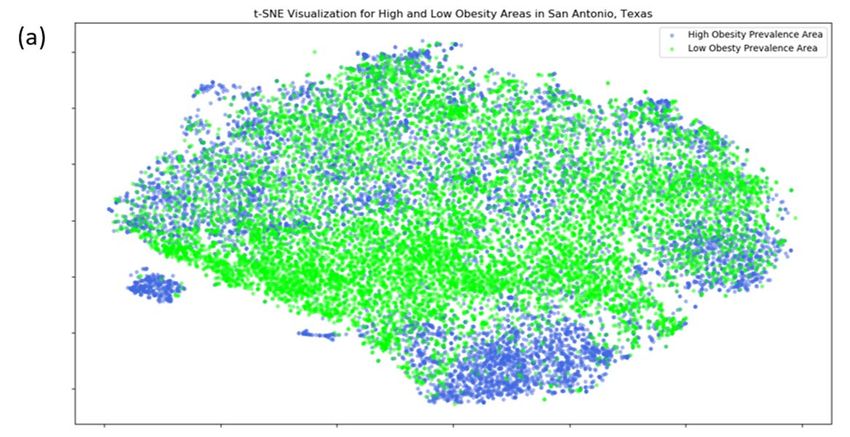
Deep Neural Network Model

                Data extracted from satellite images have been used in several health-related applications

                ranging from infectious disease monitoring to estimating socioeconomic indicators such as,

                poverty5-7. To extract information from the 150,000 satellite images, we used a convolutional

                neural network (CNN), which is the state-of-art method for most computer vision tasks such as

                object recognition, scene labelling, image segmentation and pose estimation. More recently,

                CNNs have also been trained in image recognition for skin cancer, diagnosis of plant diseases

                and classification of urban landscapes8-10.

                To train a CNN from scratch to differentiate between regions with low and high obesity

                prevalence, we need a large corpus consisting of millions of labelled images. However, such

                training data is unavailable. Instead, we used a transfer learning approach (see eFigure 1), which

                involves applying a previously trained network to our dataset of unlabeled images to make

                inferences. We used a network, VGG-CNN-F, which has been previously trained (hereafter

                referred to as, pre-trained) for object recognition on the ILSVRC-2012 challenge dataset (subset

                of ImageNet database) and is freely available to the research community11,14. The trained

                network achieved 16.7% top-5 error on the challenge test set. This implies that the network is

                able to identify the correct class for every image within its top 5 predictions or predictions with

                highest probability. The network has helped achieve breakthroughs in other image recognition

                tasks through transfer learning.

                The convolutional neural network consists of five convolutional layers and three fully connected

                layers. Each convolutional layer is composed of several two-dimensional filters which activate

                                                                    © Maharana A et al. JAMA Network Open.

Downloaded From: https://jamanetwork.com/ on 06/02/2021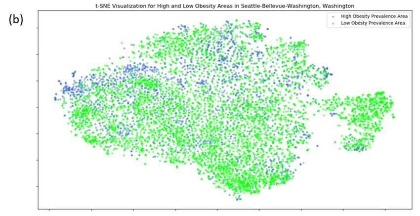
the features required for classifying an object correctly. During training, the neural network

                learns to extract gradients, edges and patterns that aid in accurate object detection. The fully

                connected layers further process these features and convert them into single dimensional vectors.

                The output layer (final fully connected layer) is originally designed for classifying between 1000

                object categories. Essentially, this neural network transforms a large two-dimensional image into

                a single vector of fixed dimension, containing only the most important descriptors of the image.

                This feature vector is extracted by deploying the network and making a forward pass through it

                for each image. It has been shown that these descriptors can be used with linear classifiers or

                regression models to perform tasks that are much different from object recognition12. We employ

                this technique to transform satellite images of dimension 224x224 into a feature vector of length

                4096, taken from the seventh hidden layer or second fully-connected layer of the VGG-CNN-F

                network.

                We also make a forward pass through the network for some images and examine the output maps

                from convolutional layers of the CNN, to see if built environment features are being highlighted

                by these filters and transmitted to the succeeding layers. The output maps are single channel

                images which can be plotted and compared to the original image for interpretation of the outputs.

                The results from this process are visualized in Figure 1.

                To investigate whether our approach could differentiate between images from areas with low and

                high obesity prevalence, we extracted the 4096-dimensional feature vectors from the second

                fully connected layer of VGG-CNN-F for each image and projected these vectors onto a 2-

                dimensional space via t-distributed stochastic neighbor embedding (t-SNE). t-SNE is a non-

                                                                    © Maharana A et al. JAMA Network Open.

Downloaded From: https://jamanetwork.com/ on 06/02/2021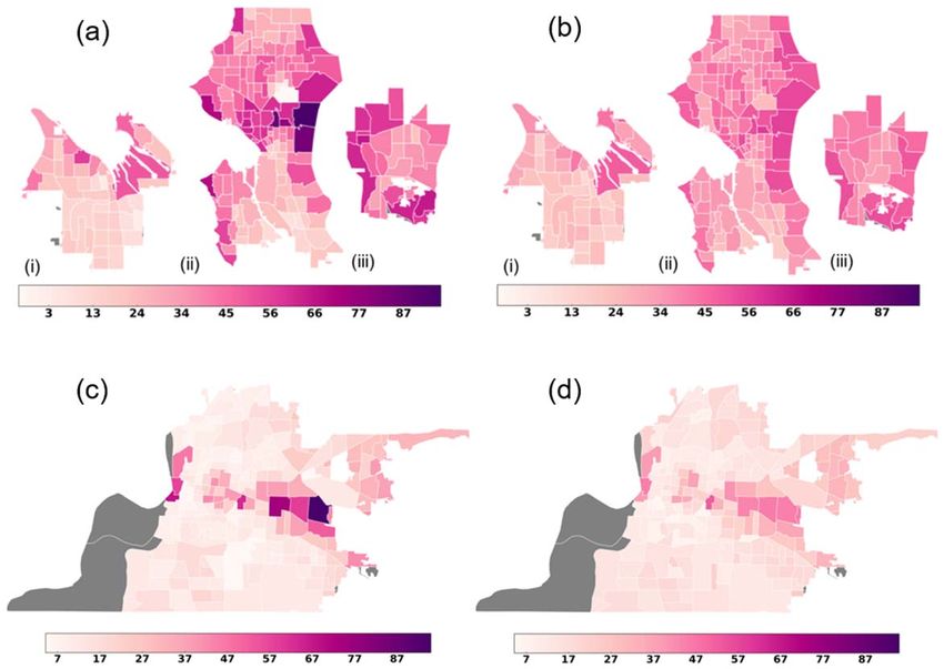
linear dimensionality reduction algorithm which has been known to preserve local

                neighborhoods at the expense of global structure15. It can be implemented using various metrics

                for measuring distance between two vectors; we used the Euclidean distance. We also fit a 3-

                component Gaussian mixture model to tract-level obesity prevalence data in order to divide

                census tracts of a city into low, and high obesity areas. All images belonging to a high obesity

                census tract were tagged as high obesity areas for the purpose of visualization, similarly for low

                obesity census tracts. Further, the mean feature vector for a census tract is computed by taking

                the average of the vectors for all satellite images belonging to that particular census tract.

                We observe well-formed clusters for low and high obesity prevalence in the visualization for San

                Antonio, showing that built environment features in these areas are distinct (eFigure 3). The

                Gaussian distribution means for census tracts in San Antonio with low and high obesity

                prevalence are 26.7 and 38.4, respectively. In contrast, the Gaussian distribution means for

                census tracts in Seattle-Tacoma-Bellevue with low and high obesity prevalence are 20.6 and 31.9

                only, making Seattle an area with low obesity prevalence. This is reflected in the t-SNE

                visualization for Seattle - the high obesity labelled data points are outnumbered and do not form

                distinct clusters within themselves. The clustering of images in eFigure 3, demonstrates that our

                approach can differentiate between images from census tracts with low and high obesity

                prevalence.

                Regression Modeling

                We conducted three different sets of analyses. Our first aim was to quantify the association

                between the features of the built environment and obesity prevalence at the census tract level.

                                                                     © Maharana A et al. JAMA Network Open.

Downloaded From: https://jamanetwork.com/ on 06/02/2021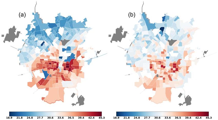
We assessed how much of the variation in obesity prevalence across all census tracts is explained

                by features of the built environment extracted from satellite images. Since the data contained a

                large number of features (n=4,096), we applied Elastic Net – a regularization and variable

                selection technique. A major benefit of Elastic Net is that it combines the advantages of Ridge

                regression and Least Absolute Shrinkage and Selection Operator (LASSO); insignificant

                covariates are eliminated, while correlated variables that are significant are maintained13. Next,

                we evaluated how well our model predicts obesity prevalence across all cities by splitting the

                data into two sets – a random sample representing sixty percent of the data for fitting and the

                remaining forty percent for model evaluation.

                Our second aim was to quantify the association between the neighborhood density of places of

                interest (such as, fast food outlets and recreational facilities) to obesity prevalence. We used the

                same process for variable selection and regression modeling as previously described. We then

                compared the model coefficient of determination (R2), root mean squared error (RMSE) and

                Pearson correlation between the actual and estimated observations to our previous results on

                estimating obesity using data on the built environment extracted from satellite images.

                Lastly, we fit separate models to quantify how well the features of the built environment

                extracted from satellite images predict socioeconomic variables, such as per capita income. This

                analysis was undertaken because obesity prevalence tends to correlate with socioeconomic status

                and we wanted to investigate if this could partially explain the performance of our models in

                predicting obesity prevalence.

                                                                     © Maharana A et al. JAMA Network Open.

Downloaded From: https://jamanetwork.com/ on 06/02/2021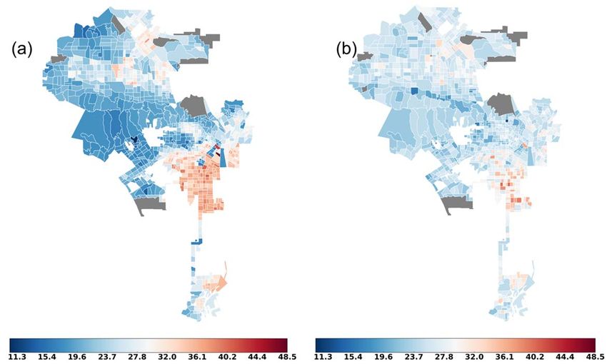
We used the R statistical software for all the regression modeling16. Five-fold cross validation

                was applied to models for all regions except Memphis, for which we used a three-fold cross

                validation because the sample size was less than 200, which limits the number of data points

                used in each fold. To prevent over-fitting, we also limited the number of selected features to be

                less than or equal to the number of census of tracts.

                                                                    © Maharana A et al. JAMA Network Open.

Downloaded From: https://jamanetwork.com/ on 06/02/2021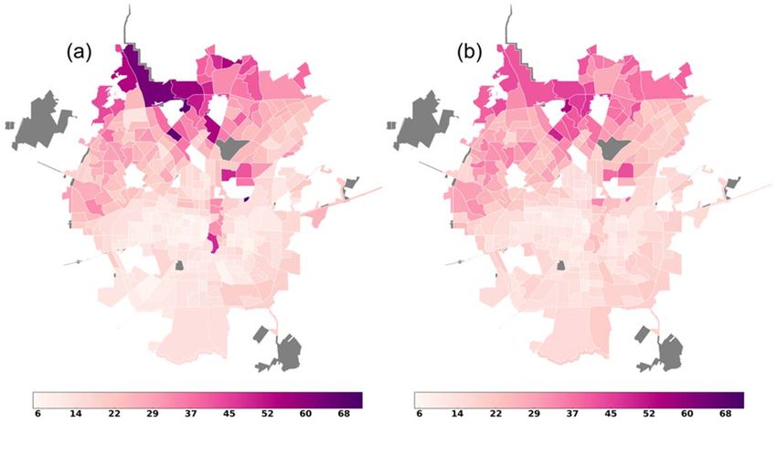
eTable 1. Places of Interest

                Accounting             Car Wash           Gas Station             Lodging           Police

                Airport                Casino             General Contractor      Meal Delivery     Post Office

                Amusement                                 Grocery or                                Real Estate
                                       Cemetery                                   Meal Takeaway
                Park                                      Supermarket                               Agency

                Aquarium               Church             Gym                     Mosque            Restaurant

                                                                                                    Roofing
                Art Gallery            City Hall          Hair Care               Movie Rental
                                                                                                    Contractor

                ATM                    Clothing Store     Hardware Store          Movie Theater     RV Park

                                       Convenience                                Moving
                Bakery                                    Health                                    School
                                       Store                                      Company

                Bank                   Courthouse         Hindu Temple            Museum            Shoe Store

                Bar                    Dentist            Home Goods Store        Natural Feature   Shopping Mall

                                       Department
                Beauty Salon                              Hospital                Neighborhood      Spa
                                       Store

                Bicycle Store          Doctor             Insurance Agency        Night Club        Stadium

                Book Store             Electrician        Jewelry Store           Painter           Storage

                                       Electronics
                Bowling Alley                             Laundry                 Park              Synagogue
                                       Store

                Bus Station            Embassy            Lawyer                  Parking           Taxi Stand

                Cafe                   Finance            Library                 Pet Store         Train Station

                Campground             Fire Station       Light Rail Station      Pharmacy          Transit Station

                Car Dealer             Florist            Liquor Store            Physiotherapist   Travel Agency

                                                                         © Maharana A et al. JAMA Network Open.

Downloaded From: https://jamanetwork.com/ on 06/02/2021
Local Government Place of
Car Rental Funeral Home University
Office Worship
Car Repair Furniture Store Locksmith Plumber Veterinary Care
Zoo
© Maharana A et al. JAMA Network Open.
Downloaded From: https://jamanetwork.com/ on 06/02/2021eTable 2. Demographic and Obesity Data
Bellevue Seattle Tacoma Los Memphis San
Angeles Antonio
2010 122,363 608,660 198,397 3,792,621 646,889 1,327,407
Population
Median age 38.5 36.1 35.1 34.1 33.0 32.7
(years)
18 years and 96,410 515,147 152,760 2,918,096 478,921 971,407
over (78.8%) (84.6%) (77.0%) (76.9%) (74.0%) (73.2%)
Male 48,020 256,561 74,539 1,441,341 221,992 466,126
(39.2%) (42.2%) (37.6%) (38.0%) (34.3%) (35.1%)
Female 48,390 258,586 78,221 1,476,755 256,929 505,281
(39.5%) (42.5%) (39.4%) (38.9%) (39.7%) (38.1%)
Income (per 50,405 44,167 26,805 28,320 21,909 22,784
capita,
2014)*
Obesity
Crude 16.3 (95% 19.2 (95% 24.6 (95% 21.1 (95% 29.3 (95% 32.4 (95%
prevalence CI, 16.2- CI, 19.2- CI, 24.6- CI, 21.1- CI, 29.2- CI, 32.4-
16.3) 19.3) 24.7) 21.1) 29.4) 32.5)
Age-adjusted 18.8 (95% 22.4 (95% 30.8 (95% 26.7 (95% 36.3 (95% 32.9 (95%
prevalence CI, 18.6- CI, 22.3- CI, 30.6- CI, 26.7- CI, 36.2- CI, 32.8-
18.9) 22.5) 31) 26.8) 36.5) 32.9)
© Maharana A et al. JAMA Network Open.
Downloaded From: https://jamanetwork.com/ on 06/02/2021*American Community Survey, 2014 5-year estimate.
eFigure 1. Illustration of Transfer Learning Approach
Let classification of objects from the ImageNet dataset be Domain A. The model trained for
domain A has learnt how to interpret an image. We use this knowledge acquired by the model to
understand satellite images. When the satellite images are fed as input to the model, we receive
feature maps that encode this knowledge. These feature maps are used in a regression model to
predict obesity values which is domain B. (Left composite image courtesy of ImageNet:
http://image-net.org/)
© Maharana A et al. JAMA Network Open.
Downloaded From: https://jamanetwork.com/ on 06/02/2021eFigure 2. VGG-CNN-F Convolutional NN Architecture
We have used the 8-layer VGG-CNN-F convolutional neural network for our project. In this
architecture, the first five layers are a five-fold repetition of this arrangement: pooling layer->ReLU layer> Those layers are represented in blue. The next 3 layers
(represented in green) are fully connected layers. (Left composite image courtesy of ImageNet:
http://image-net.org/)
© Maharana A et al. JAMA Network Open.
Downloaded From: https://jamanetwork.com/ on 06/02/2021eFigure 3. t-SNE Visualization of Features Extracted From VGG-CNN-F for Satellite
Imagery
(a) San Antonio, Texas and (b) Seattle-Tacoma-Bellevue area, Washington.
© Maharana A et al. JAMA Network Open.
Downloaded From: https://jamanetwork.com/ on 06/02/2021eFigure 4. Actual Obesity Prevalence and Cross-validated Model Estimates of Obesity
Prevalence
(a) actual and (b) cross-validated estimates of obesity prevalence for Bellevue (i), Seattle (ii) and
Tacoma (iii), Washington based on the density of places of interest data. These cities are
collectively referred to as Seattle in the manuscript. We do not have data for the gray shaded
regions.
© Maharana A et al. JAMA Network Open.
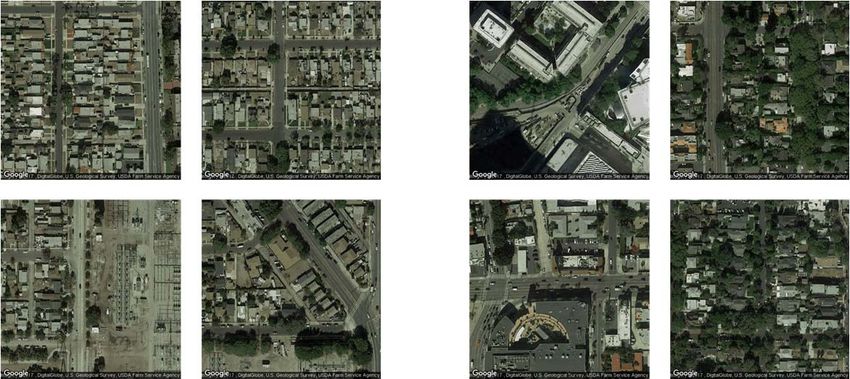
Downloaded From: https://jamanetwork.com/ on 06/02/2021eFigure 5. Google Satellite Images for Seattle Showing Locations With Low and High
Obesity Prevalence, Respectively
(Left grouping) Census tracts containing affluent neighborhoods (close to waterfront, swimming
pool in apartment complex), waterfront businesses and downtowns are classified as low obesity
areas in Seattle-Tacoma-Bellevue area. (Right grouping) Census tracts with small population
density and less urbanized footprint are classified as high obesity areas in Seattle-Tacoma-
Bellevue area.
© Maharana A et al. JAMA Network Open.
Downloaded From: https://jamanetwork.com/ on 06/02/2021eFigure 6. Actual Obesity Prevalence and Cross-validated Model Estimates of Obesity
Prevalence
(a) actual and (b) cross-validated estimates of obesity prevalence for San Antonio, Texas based
on the density of places of interest data. Unlike Seattle, the places of interest data appear to
capture the variability in obesity prevalence across census tracts. We do not have data for the
gray shaded regions.
© Maharana A et al. JAMA Network Open.
Downloaded From: https://jamanetwork.com/ on 06/02/2021eFigure 7. Google Satellite Images for San Antonio Showing Locations With Low and High
Obesity Prevalence, Respectively
(Top Row) Census Tract 48029190400 – Images show dense green cover in residential areas and
school building. (Bottom Row) Census Tract 48029130402 –The neighborhoods are dominated
by larger roadways.
© Maharana A et al. JAMA Network Open.
Downloaded From: https://jamanetwork.com/ on 06/02/2021eFigure 8. Actual Obesity Prevalence and Cross-validated Model Estimates of Obesity
Prevalence
(a) actual and (b) cross-validated estimates of obesity prevalence for Memphis, Tennessee based
on the density of places of interest data. The places of interest data capture the variability in
neighborhood obesity prevalence for Memphis much better than it does for Seattle and Los
Angeles (below), where the overall obesity prevalence is lower. We do not have data for the gray
shaded regions.
© Maharana A et al. JAMA Network Open.
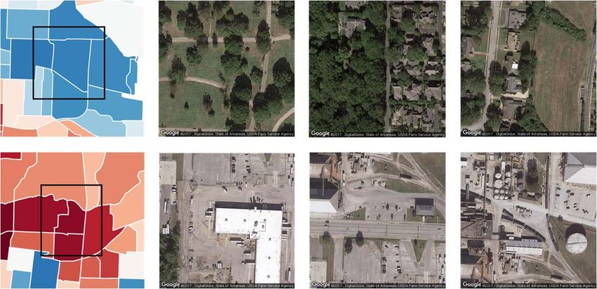
Downloaded From: https://jamanetwork.com/ on 06/02/2021eFigure 9. Google Satellite Images for Memphis Showing Locations With Low and High
Obesity Prevalence, Respectively
(Top Row) Census Tract 47157009600 – Images show green cover in neighborhood and
walkways in field. (Bottom Row) Census Tract 47157000800 – Industrial area, presence of
vehicles and sparse greenery.
© Maharana A et al. JAMA Network Open.
Downloaded From: https://jamanetwork.com/ on 06/02/2021eFigure 10. Actual Obesity Prevalence and Cross-validated Model Estimates of Obesity
Prevalence
(a) actual and (b) cross-validated estimates of obesity prevalence for Los Angeles, California
based on the density of places of interest data.
© Maharana A et al. JAMA Network Open.
Downloaded From: https://jamanetwork.com/ on 06/02/2021eFigure 11. Google Satellite Images for Los Angeles Showing Locations With Low and
High Obesity Prevalence, Respectively
(Left grouping) High obesity census tracts are characterized by densely packed neighborhoods
and less greenness. (Right grouping) Low obesity census tracts consist of mostly residential
areas with more street greenness.
© Maharana A et al. JAMA Network Open.
Downloaded From: https://jamanetwork.com/ on 06/02/2021eFigure 12. Out-of-Sample Predictions of Obesity Prevalence Plotted Against Actual
Obesity Prevalence
Obesity prevalence plotted against (a) Los Angeles, California (b) Memphis, Tennessee (c)
San Antonio, Texas, (d) Seattle, Washington based on places of interest data.
© Maharana A et al. JAMA Network Open.
Downloaded From: https://jamanetwork.com/ on 06/02/2021eFigure 13. Cross-validated Model Estimates of Per Capita Income Plotted Against Actual
Per Capita Income
Actual per capita income for (a) Los Angeles, California (b) San Antonio, Texas (c) Seattle,
Washington (d) Memphis, Tennessee
© Maharana A et al. JAMA Network Open.
Downloaded From: https://jamanetwork.com/ on 06/02/2021eFigure 14. Out-of-Sample Model Predictions of Per Capita Income Plotted Against Actual
Per Capita Income
Plotted against actual per capita income for (a) Los Angeles, California (b) Memphis,
Tennessee (c) San Antonio, Texas and (d) Seattle, Washington
© Maharana A et al. JAMA Network Open.
Downloaded From: https://jamanetwork.com/ on 06/02/2021eFigure 15. Actual Per Capita Income and Cross-validated Model Estimates of Per Capita
Income
© Maharana A et al. JAMA Network Open.
Downloaded From: https://jamanetwork.com/ on 06/02/2021(a), (c) actual and (b), (d) cross-validated estimates of per capita income for San Antonio, Texas
and Los Angeles, California respectively, based on the features extracted from satellite images.
The unit is in thousands of dollars.
© Maharana A et al. JAMA Network Open.
Downloaded From: https://jamanetwork.com/ on 06/02/2021eFigure 16. Actual Per Capita Income and Cross-validated Model Estimates of Per Capita
Income
(a), (c) actual and (b), (d) cross-validated estimates of per capita income for Bellevue (i), Seattle
(ii) and Tacoma (iii), Washington, and Memphis, Tennessee respectively, based on the features
extracted from satellite images. The unit is in thousands of dollars.
© Maharana A et al. JAMA Network Open.
Downloaded From: https://jamanetwork.com/ on 06/02/2021eReferences
1. CDC (2017) 500 Cities: Local Data for Better Health. Available at:
https://www.cdc.gov/500cities/ [Accessed September 13, 2017].
2. CDC (2016) Overweight & Obesity: Adult Obesity Facts. Available at:
https://www.cdc.gov/obesity/data/adult.html [Accessed May 19, 2017].
3. CDC (2016) 500 Cities: Local Data for Better Health. Unhealthy Behaviors. Available at:
https://www.cdc.gov/500cities/definitions/unhealthy-behaviors.htm [Accessed September
13, 2017].
4. The State of Obesity. Obesity Rates & Trends - Adult Obesity in the United States (2017)
Available at: https://stateofobesity.org/rates/ [Accessed October 14, 2017].
5. Nsoesie EO, Butler P, Ramakrishnan N, Mekaru SR, Brownstein JS (2015) Monitoring
Disease Trends using Hospital Traffic Data from High Resolution Satellite Imagery: A
Feasibility Study. Sci Rep 5:9112.
6. Karnieli A, Gilad U, Ponzet M, Svoray T, Mirzadinov R, Fedorina O (2008) Assessing
land-cover change and degradation in the Central Asian deserts using satellite image
processing and geostatistical methods. J Arid Environ 72(11):2093–2105.
7. Jean N, Burke M, Xie M, Davis WM, Lobell DB, Ermon S (2016) Combining satellite
imagery and machine learning to predict poverty. Science 353(6301):790–794.
8. Mohanty SP, Hughes DP, Salathé M (2016) Using deep learning for image-based plant
disease detection. Front Plant Sci 7.
9. Esteva A, Kuprel B, Novoa RA, Ko J, Swetter SM, Blau HM, Thrun S (2017)
Dermatologist-level classification of skin cancer with deep neural networks. Nature
© Maharana A et al. JAMA Network Open.
Downloaded From: https://jamanetwork.com/ on 06/02/2021542(7639):115–118.
10. Albert A, Kaur J, Gonzalez M (2017) Using convolutional networks and satellite imagery
to identify patterns in urban environments at a large scale. ArXiv Prepr ArXiv170402965.
11. Deng J, Dong W, Socher R, Li L-J, Li K, Fei-Fei L (2009) Imagenet: A large-scale
hierarchical image database. Computer Vision and Pattern Recognition, 2009. CVPR
2009. IEEE Conference on (IEEE), pp 248–255.
12. Sharif Razavian A, Azizpour H, Sullivan J, Carlsson S (2014) CNN features off-the-
shelf: an astounding baseline for recognition. Proceedings of the IEEE Conference on
Computer Vision and Pattern Recognition Workshops, pp 806–813.
13. Friedman J, Hastie T, Tibshirani R (2001) The elements of statistical learning (Springer
series in statistics Springer, Berlin).
14. Chatfield K, Simonyan K, Vedaldi A, Zisserman A (2014) Return of the devil in the
details: Delving deep into convolutional nets. ArXiv Prepr ArXiv 14053531.
15. Maaten L van der, Hinton G. Visualizing data using t-SNE. J Mach Learn Res.
2008;9(Nov):2579–2605.
16. R Core Team (2013). R: A language and environment for statistical computing. R
Foundation for Statistical Computing, Vienna, Austria. URL http://www.R-project.org/.
© Maharana A et al. JAMA Network Open.
Downloaded From: https://jamanetwork.com/ on 06/02/2021You can also read