Forecasting Daily Volatility of Stock Price Index Using Daily Returns and Realized Volatility
←
→
Page content transcription
If your browser does not render page correctly, please read the page content below
HIAS-E-104

            Forecasting Daily Volatility of Stock Price Index
                 Using Daily Returns and Realized Volatility
                       Makoto Takahashi(a), Toshiaki Watanabe(b), Yasuhiro Omori(c)

                          (a) Faculty of Business Administration, Hosei University, Japan
                        (b) Institute of Economic Research, Hitotsubashi University, Japan
                               (c) Faculty of Economics, University of Tokyo, Japan

                                                   January, 2021

Hitotsubashi Institute for Advanced Study, Hitotsubashi University
2-1, Naka, Kunitachi, Tokyo 186-8601, Japan
tel:+81 42 580 8668 http://hias.hit-u.ac.jp/

HIAS discussion papers can be downloaded without charge from:
http://hdl.handle.net/10086/27202
https://ideas.repec.org/s/hit/hiasdp.html

All rights reserved.
Forecasting Daily Volatility of Stock Price Index

                             Using Daily Returns and Realized Volatility

                     Makoto Takahashi1 , Toshiaki Watanabe∗ 2 , and Yasuhiro Omori3
                         1
                             Faculty of Business Administration, Hosei University, Japan
                     2
                         Institute of Economic Research, Hitotsubashi University, Japan
                                 3
                                     Faculty of Economics, University of Tokyo, Japan

                                                     January 4, 2021

                                                         Abstract

         This paper compares the volatility predictive abilities of some time-varying volatility models such as the

      stochastic volatility (SV) and exponential GARCH (EGARCH) models using daily returns, the heterogeneous au-

      toregressive (HAR) model using daily realized volatility (RV) and the realized SV (RSV) and realized EGARCH

      (REGARCH) models using the both. The data are the daily return and RV of Dow Jones Industrial Aver-

      age (DJIA) in US and Nikkei 225 (N225) in Japan. All models are extended to accommodate the well-known

      phenomenon in stock markets of a negative correlation between today’s return and tomorrow’s volatility. We

      estimate the HAR model by the ordinary least squares (OLS) and the EGARCH and REGARCH models by

      the quasi-maximum likelihood (QML) method. Since it is not straightforward to evaluate the likelihood of the

      SV and RSV models, we apply a Bayesian estimation via Markov chain Monte Carlo (MCMC) to them. By

      conducting predictive ability tests and analyses based on model confidence sets, we confirm that the models us-

      ing RV outperform the models without RV, that is, the RV provides useful information on forecasting volatility.

      Moreover, we find that the realized SV model performs best and the HAR model can compete with it. The

      cumulative loss analysis suggests that the differences of the predictive abilities among the models are partly

      caused by the rise of volatility.

      JEL classification: C11, C22, C53, C58, G17.

      Keywords: Exponential GARCH (EGARCH) model; Heterogeneous autoregressive (HAR) model; Markov chain

      Monte Carlo (MCMC); Realized volatility; Stochastic volatility; Volatility forecasting.

  ∗ Corresponding author. Institute of Economic Research, Hitotsubashi University, 2-1 Naka, Kunitachi, Tokyo 186-8603 Japan.

E-mail address: watanabe@ier.hit-u.ac.jp

                                                             1
1     Introduction

Few would dispute the fact that financial volatility changes stochastically over time, so that it is important to forecast

time-varying volatility for financial risk management. Time-varying volatility used to be estimated and forecasted

by applying generalized autoregressive conditionally heteroskedasticity (GARCH) and stochastic volatility (SV)

models to financial returns. These models are consistent with the volatility clustering, i.e., high persistence in

volatility and has been extended to accommodate the phenomenon called volatility asymmetry or leverage effect,

i.e., negative correlation between today’s return and tomorrow’s volatility observed in stock markets. One of such

extensions is the exponential GARCH (EGARCH) model proposed by Nelson (1991).

    In recent years, realized volatility (RV) has replaced these models for volatility estimation. Daily RV is calculated

as the sum of squared intraday returns over a day. Andersen and Benzoni (2009) and McAleer and Medeiros (2008)
provide reviews of RV. To predict volatility using RV, we must model the dynamics of RV. Many researchers including

Andersen et al. (2001a,b, 2003) have documented that daily RV may follow a long-memory process, so that they use

autoregressive fractionally integrated moving average (ARFIMA) models. See Beran (1994) for long-memory and

ARFIMA models. The model used more widely for the dynamics of RV is the heterogeneous autoregressive (HAR)

model proposed by Corsi (2009), which is not a long-memory model but is known to approximate a long-memory

process well.

    Two types of hybrid models have been proposed. One is the realized SV (RSV) model proposed by Takahashi et

al. (2009) and the other is the realized GARCH (RGARCH) model proposed by Hansen et al. (2012). RV is subject

to the bias caused by microstructure noise and non-trading hours. There are some methods for mitigating the bias

in RV. See Ait-Sahalia and Mykland (2009), Ubukata and Watanabe (2014) and Liu et al. (2015) for such methods.

The RSV and RGARCH models model returns and RV jointly taking account of the bias in RV. Hansen and Hunag

(2016) extend the RGARCH model to the realized EGARCH (REGARCH) model, which is more general than the

RGARCH model.

    This paper compares the volatility predictive abilities of the SV, EGARCH, HAR, RSV and REGARCH models.

The data we use are the daily return and RV of Dow Jones Industrial Average (DJIA) in US and Nikkei 225 (N225)

in Japan. As mentioned above, volatility asymmetry is a well-known phenomenon for stock indices. The EGARCH
and REGARCH models can capture this phenomenon. Similarly, we extend the other models by taking it into

account. We use daily return for the SV and EGARCH models, daily RV for the HAR model and the both for the

RSV and REGARCH models. We estimate the HAR model by the ordinary least squares (OLS) and the EGARCH

and REGARCH models by the quasi-maximum likelihood (QML) method. Since it is not straightforward to evaluate

the likelihood of the SV and RSV models, we apply a Bayesian estimation via Markov chain Monte Carlo (MCMC)

to them.

    The problem in the comparison of volatility predictive abilities is that the true volatility is unobserved. Patton

(2011) shows that the mean squared error (MSE) and the quasi-likelihood (QLIKE) are robust loss functions in

                                                            2
the sense that they would lead to the same ranking as the one when the true volatility are used if the proxy for
the true volatility is a conditionally unbiased estimator of the true volatility. We use the MSE and QLIKE as
loss functions for the comparison of volatility predictive abilities. Although Koopman et al. (2005) compares the
volatility predictive abilities among several models, they do not include the HAR, RSV and REGARCH models
and the comparison method is different from ours.
The realized SV model gives the lowest MSE and QLIKE values for both DJIA and N225. Implementing the
predictive ability test of Giacomini and White (2006) and undertaking an analysis based on the model confidence
set of Hansen et al. (2011), we confirm that the models using RV outperform the models without RV. That is, the
RV provides the useful information on forecasting volatility. Among the models using RV, we find that the RSV
model performs best and the HAR model can compete with it. The cumulative loss analysis suggests that the
differences of the predictive abilities among the models are partly caused by the rise of volatility.
The rest of the paper proceeds as follows. Sections 2 reviews the SV and RSV models and explains the Bayesian
method via MCMC for estimating the parameters in these models and forecasting volatility. Section 3 reviews the
HAR, EGARCH and REGARCH models. Section 4 applies all models to daily return and RV of DJIA and N225
and compares the volatility predictive abilities. Section 5 concludes.
2 Stochastic Volatility and Realized Stochastic Volatility Models
In this section, we review the SV and RSV models and explain the Bayesian method via MCMC for estimating the
parameters in these models and forecasting volatility.
2.1 Stochastic Volatility Model
The SV model is a well-known model to describe the time-varying volatilities of the asset returns. First, define the
daily return of the asset as yt = log pt − log pt−1 where pt denotes the closing price for the day t. Let ht denote
the logarithm of the volatility. The log volatility ht is a latent variable and assumed to follow the stationary first
order autoregressive (AR(1)) process with the autoregressive parameter ϕ and mean µ. The absolute value of ϕ is
assumed to be less than one for the stationarity of the log volatility. Given ht at time t, the SV model is defined as
follows:
yt = ϵt exp(ht /2), t = 1, . . . , n, (1)
ht+1 = µ + ϕ(ht − µ) + ηt , t = 1, . . . , n − 1, |ϕ| < 1, (2)
h1 ∼ N (µ, ση2 /(1 − ϕ2 )),
ϵt 1 ρση
∼ N (0, Σ), Σ = ,
ηt ρση ση2
3where N (a, A) denotes normal distribution with mean a and covariance matrix A. We assume the stationary
distribution for the initial log latent volatility h1 . The AR(1) process for ht ’s is supposed to describe the volatility
clustering, which refers to the persistence in the volatilities where the large changes in price tend to cluster together.
The disturbance vector (ϵt , ηt )′ is assumed to follow the bivariate normal distribution with mean 0 and covariance
matrix Σ. We consider the correlation ρ between ϵt and ηt (equivalently, yt and ht+1 ). The negative correlation
(ρ < 0) refers to the volatility asymmetry or the leverage effect which implies the decrease in yt followed by the
increase in ht+1 .
The SV model defined by (1) and (2) is a nonlinear Gaussian state space model with many latent variables,
making it difficult to evaluate the likelihood function given the parameter ϑ = (µ, ϕ, ση2 , ρ) and to implement the
maximum likelihood estimation. To overcome this difficulty, we take Bayesian approach to estimate parameters
using Markov chain Monte Carlo (MCMC) simulation as in the previous literature. For the prior distribution of ϑ,
we assume
µ ∼ N (mµ , s2µ ), ϕ ∼ π(ϕ), ρ ∼ π(ρ), ση2 ∼ IG(nη /2, Sη /2),
where IG(a, b) denotes inverse gamma distribution with shape parameter a and rate parameter b so that
( )
( )−( n2η +1) Sη
π(ση2 ) ∝ ση2 exp − 2 ,
2ση
and ϕ and ρ are assumed to follow prior distributions with probability densities π(ϕ) and π(ρ), respectively. The
parameters of the prior distributions (mµ , s2µ , nη , Sη ) are hyperparameters and are chosen to be some constants to
reflect the prior information regarding parameters.
Let π(ϑ) denote the joint prior probability density of ϑ, and let y = (y1 , . . . , yn )′ and h = (h1 , . . . , hn )′ . Further,
let f (y, h|ϑ) denote the likelihood of y and h given ϑ. Then, the joint posterior probability density π(ϑ, h|y) is
given by
π(ϑ, h|y)
∝ f (y, h|ϑ)π(ϑ)
{ }
1∑ 1∑ 2 √
n n
yt exp(−ht ) × 1 − ϕ2 × (ση2 )−( 2 ) × (1 − ρ2 )− 2
n n−1
∝ exp − ht −
2 t=1 2 t=1
{ }
(1 − ϕ2 )(h1 − µ)2 ∑ (ht+1 − (1 − ϕ)µ − ϕht − ρση exp(−ht /2)yt )2
n−1
× exp − −
2ση2 t=1
2ση2 (1 − ρ2 )
{ } { }
n
2 −( 2η +1) (µ − mµ )2 Sη
×π(ϕ) × π(ρ) × (ση ) exp − exp − 2 . (3)
2s2µ 2ση
We implement MCMC simulations in seven blocks:
41. Initialize ϑ and h.
2. Generate µ|ϑ\µ , h, y.
3. Generate ϕ|ϑ\ϕ , h, y.
4. Generate ση2 |ϑ\ση2 , h, y.
5. Generate ρ|ϑ\ρ , h, y.
6. Generate h|ϑ, y.
7. Go to Step 2.
where ϑ\x denotes ϑ excluding its component x. Since ht is highly correlated with ht+1 and ht−1 , the simple
MCMC step for h results in the inefficient sampling. The efficient sampling algorithms for h are proposed such as
the mixture sampler based on the approximation by the mixture of normal distributions (Omori et al. (2007)) and
the block sampler (Omori and Watanabe (2008)).
2.2 Realized Volatility
In the SV model, the volatility exp(ht ) has been considered as a latent variable since ht is unobserved. Recently,
the high frequency data has become widely available and the realized volatility (RV) is proposed as the estimator
of the true volatility using the intraday data. We first define the true volatility for day t. Let p(s) denote the
logarithm of the price of the asset at time s and assume it follows the continuous time diffusion process given by
dp(s) = µ(s)ds + σ(s)dW (s), (4)
where µ(s), σ 2 (s), and W (s) are the drift, the volatility, and the Wiener process, respectively. Let t denote the
market closing time on day t. Then, the true volatility for day t is defined as the volatility between t − 1 and t:
∫ t
IVt = σ 2 (s)ds, (5)
t−1
which is also called the integrated volatility. Suppose we have n intraday observations for the day t given by
{ }
rt−1+1/n , rt−1+2/n , . . . , rt . Then the realized volatility, the estimator of IVt , is defined by
∑
n
2
RVt = rt−1+i/n . (6)
i=1
Under some conditions, it can be shown that RVt converges to IVt as n → ∞. However, those conditions are not
satisfied in practice by high frequency data, and the estimator is known to have a bias. For example, if we ignore
5the non-trading hours to compute the realized volatility, we underestimate the true volatility. Moreover, the actual
asset prices are observed with the microstructure noise, which results in the autocorrelations in the asset returns
and violate these assumptions. The effect of the microstructure noise is known to become larger as the time interval
between observed prices becomes smaller. The optimal time intervals to compute the RV is investigated in the
literature (Ait-Sahalia, Mykland and Zhang (2005), Bandi and Russell (2006, 2008), Liu et al. (2015)). Alternative
estimators are also proposed such as two (multi) scale estimator (Zhang, Mykland and Ait-Sahalia (2005), Zhang
(2006)) and realized kernel (Barndorff-Nielsen et al. (2008, 2009)). To deal with the non-trading hours, Hansen and
Lunde (2005) proposed to adjust the RVt as follows:
∑T
1∑
T
t=1 (yt − y)
2
(c)
RVt = cRVt , c= ∑T , y= yt , (7)
t=1 RVt
T t=1
(c)
where RVt represents the realized volatility when we ignore the non-trading hours. The average of RVt is set
equal to the sample variance of the daily returns. On the other hand, the RSV model proposed in Takahashi et
al. (2009) adjusts the bias of the RV by estimating the model parameter for the bias correction as we shall see in
Section 2.3.
2.3 Realized SV Model
Takahashi et al. (2009) introduces the additional source of information regarding the true volatility. In addition to
the measurement equation of daily return yt , they consider that of log RV, that is, xt = log RVt . Let ht denote the
logarithm of the true volatility, ht = log IVt . The realized stochastic volatility (RSV) model is defined as
yt = exp(ht /2)ϵt , t = 1, . . . , n, (8)
ht+1 = µ + ϕ(ht − µ) + ηt , t = 1, . . . , n − 1, |ϕ| < 1, (9)
xt = ξ + ht + ut , t = 1, . . . , n, (10)
h1 ∼ N (0, ση2 /(1 − ϕ2 )),
ϵt 1 ρση 0
ηt 0
∼ N (0, Σ) , Σ = ρση ση2 , (11)
ut 0 0 σu2
where ut is assumed to be independent of (ϵt , ηt ) for simplicity. In general, we could replace (10) by
xt = ξ + ψht + ut .
6Since, in empirical studies, it is found that this extension does not improve the forecasting performance of the
volatilities, we assume ψ = 1 as in Takahashi et al. (2009). ξ is the bias correction parameter in log RVt and ξ = 0
implies that there is no bias. If we ignore the non-trading hours to compute the RV, we underestimate IVt and
expect the negative bias. Hansen and Lunde (2006) show that the microstructure noise may result in positive or
negative bias. Thus, ξ > 0 if the bias caused by microstructure noise is positive and dominates the negative bias
caused by ignoring non-trading hours to compute the RV and ξ < 0 otherwise.
2.4 MCMC implementation for RSV models
We set ϑ = (µ, ϕ, ση2 , ρ, ξ, σu2 ) for the RSV model and let y = {yt , xt }nt=1 and h = {ht }nt=1 . We assume the prior
distribution for (µ, ϕ, ση2 , ρ) as in Section 2.1, and assume normal distribution and inverse gamma distribution for
ξ and σu2 , respectively.
µ ∼ N (mµ , s2µ ), ϕ ∼ π(ϕ), ρ ∼ π(ρ), ση2 ∼ IG(nη /2, Sη /2),
ξ ∼ N (mξ , s2ξ ), σu2 ∼ IG(nu /2, Su /2),
where (mµ , s2µ , nη , Sη , mξ , s2ξ , nu /2, Su /2) are hyperparameters. Let π(ϑ) denote the joint prior probability density
of ϑ, and let y = (y1 , . . . , yn )′ , x = (x1 , . . . , xn )′ and h = (h1 , . . . , hn )′ . Further, let f (y, x, h|ϑ) denote the
likelihood of (y, x, h) given ϑ. Then the joint posterior probability density π(ϑ, h|y, x) is given by
π(ϑ, h|y, x)
∝ f (y, x, h|ϑ)π(ϑ)
{ }
1∑ 1∑ 2 √
n n
yt exp(−ht ) × 1 − ϕ2 × (ση2 )−( 2 ) × (1 − ρ2 )− 2
n n−1
∝ exp − ht −
2 t=1 2 t=1
{ }
(1 − ϕ2 )(h1 − µ)2 ∑ (ht+1 − (1 − ϕ)µ − ϕht − ρση exp(−ht /2)yt )2
n−1
× exp − −
2ση2 t=1
2ση2 (1 − ρ2 )
{ } { }
n
2 −( 2η +1) (µ − mµ )2 Sη
×π(ϕ)π(ρ) × (ση ) exp − exp − 2
2s2µ 2ση
( n +n )
{ n }
ξ ∑ (xt − ξ − ht ) 2
(ξ − mξ )2 Su
2 − +1
×(σu ) 2
× exp − − − 2 (12)
t=1
2σu2 2s2ξ 2σu
We implement the MCMC simulation in eight blocks:
1. Initialize (µ, ϕ, ση , ρ, ξ, σu ) and h
2. Generate µ|ϕ, ση , ρ, ξ, σu , h, y, x.
3. Generate ϕ|ση , ρ, µ, ξ, σu , h, y, x.
4. Generate (ση , ρ)|ϕ, µ, ξ, σu , h, y, x.
75. Generate ξ|ϕ, ση , ρ, µ, σu , h, y, x.
6. Generate σu |ϕ, ση , ρ, µ, ξ, h, y, x.
7. Generate h|ϑ, y, x.
8. Go to Step 2.
Generation of µ. The conditional posterior distribution of µ is normal, and we generate
µ|ϕ, ση2 , h, y ∼ N (m̃µ , s̃2µ ),
where
{ }
∑
n−1
m̃µ = s̃2µ s−2
µ mµ + ση−2 (1 − ϕ )h1 + (1 −
2
ρ2 )−1 ση−2 (1 − ϕ) (ht+1 − ϕht − ȳt )
t=1
{ −2 }−1
s̃2µ = sµ + ση−2 (1 − ϕ2 ) + (1 − ρ2 )−1 ση−2 (1 − ϕ)2 (n − 1) ,
and ȳt = ρση exp(−ht /2)yt .
Generation of ϕ. The conditional posterior density of ϕ is given by
{ }
√ (1 − ϕ 2
)(h1 − µ) 2 ∑ (ht+1 − (1 − ϕ)µ − ϕht − ȳt )2
n−1
π(ϕ|·) ∝ π(ϕ) 1 − ϕ2 exp − −
2ση2 t=1
2ση2 (1 − ρ2 )
{ }
√ (ϕ − m̃ϕ )2
∝ π(ϕ) 1 − ϕ2 exp − , (13)
2s̃2ϕ
where
∑n−1
(ht+1 − µ − ȳt )(ht − µ) ση2 (1 − ρ2 )
m̃ϕ = t=1
∑n−1 , s̃2ϕ = ∑n−1 .
ρ2 (h1 − µ)2 + t=2 (ht − µ)2 ρ2 (h1 − µ)2 + t=2 (ht − µ)2
We generate ϕ using the Metropolis-Hastings (MH) algorithm. Propose a candidate ϕ† ∼ T N (−1,1) (m̃ϕ , s̃2ϕ ) where
T N (a,b) (m, s2 ) denotes normal distribution with mean m and variance s2 truncated on the interval (a, b), and
accept it wit probability
{ √ }
π(ϕ† ) 1 − ϕ†2
min √ ,1 .
π(ϕ) 1 − ϕ2
8Generation of (ση2 , ρ). The joint conditional density of (ση2 , ρ) is given by
∝ π(ση2 , ρ) × (ση2 )− 2 × (1 − ρ2 )− 2
n n−1
π(ση2 , ρ|·)
{ }
(1 − ϕ2 )(h1 − µ)2 ∑ (ht+1 − (1 − ϕ)µ − ϕht − ȳt )2
n−1
× exp − − , (14)
2ση2 t=1
2ση2 (1 − ρ2 )
where π(ση2 , ρ) denotes a prior density of (ση2 , ρ). To conduct the MH algorithm, we transform (ση2 , ρ) to ϖ =
(ϖ1 , ϖ2 )′ where ϖ1 = log ση2 , ϖ2 = log(1 + ρ) − log(1 − ρ). First, compute the mode of the conditional posterior
density π̃(ϖ|·) numerically, and denote it as ϖ̂. Then generate a candidate ϖ † ∼ N (ϖ̃, Σ̃) where
∂ log π̃(ϖ|·) ∂ log π̃(ϖ|·)
ϖ̃ = ϖ̂ + Σ̃ , Σ̃−1 = − ,
∂ϖ ϖ=ϖ̂ ∂ϖ∂ϖ ′ ϖ=ϖ̂
and accept it with probability
{ }
π(ση2† , ρ† |·)fN (ϖ|ϖ̃, Σ̃)|J(ση2 , ρ)|
min ,1 .
π(ση2 , ρ|·)fN (ϖ † |ϖ̃, Σ̃)|J(ση2† , ρ† |
where fN (x|µ, Σ) is a probability density function of a bivariate normal distribution with mean µ and covariance
matrixΣ, J(·) is a Jacobian of the transformation, and (ση2† , ρ† ) = (exp(ϖ1† ), {exp(ϖ2† ) − 1}/{exp(ϖ2† ) + 1}). If we
assume ρ = 0 (without a leverage effect), we generate ση2 ∼ IG(ñη /2, S̃η /2) where ñη = nη + n, S̃η = Sη + (1 −
∑n−1
ϕ2 )(h1 − µ)2 + t=1 {ht+1 − (1 − ϕ)µ − ϕht }2 .
Generation of ξ. The conditional posterior distribution of ξ is normal and we generate
∑n −2
σu−2 t=1 (xt − ht ) + sξ mξ
ξ|· ∼ N (m̃ξ , s̃2ξ ), m̃ξ = , s̃−2 −2 −2
ξ = nσu + sξ .
nσu−2 + s−2
ξ
Generation of σu2 . The conditional posterior distribution of σu2 is inverse gamma distribution and we generate
∑
n
σu2 |· ∼ IG(ñu /2, S̃u /2), ñu = n + nu , S̃u = (xt − ξ − ht )2 + Su .
t=1
Generation of h. For the generation of h, see Appendix.
2.5 Volatility Forecasts
To obtain the one-day ahead volatility forecasts, we follow the Bayesian sampling scheme of Takahashi et al. (2016).
Let n be the last observation used in the estimation. Then, for each sample of (ϑ, h) generated by the MCMC
92
algorithm above, we generate hn+1 from the normal distribution N (µn+1 , σn+1 ), where
µn+1 = µ + ϕ(hn − µ) + ρση yn exp(−hn /2), 2
σn+1 = (1 − ρ2 )ση2 . (15)
(i) 2
Using the sample hn+1 (i = 1, . . . , m), we compute the one-day ahead volatility forecast σ̂n+1 as follows:
1 ∑
m
2 (i)
σ̂n+1 = exp(hn+1 ). (16)
m i=1
3 Other Models
3.1 HAR Model
As mentioned, many researchers have documented that RV may follow a long-memory process and used ARFIMA
models for describing the dynamics of RV. However, the HAR model proposed by Corsi (2009) has recently been
used more widely. We extend the log version of the HAR model to accommodate the vo;atility asymmetry as
follows:
−
xt = β0 + βd xt−1 + βw xt−5:t−1 + βm xt−22:t−1 + λyt−1 + vt , vt ∼ N (0, σv2 ), (17)
where xt and xt−1 represent the log of daily RVs on days t and t − 1, respectively, and xt−5:t−1 and xt−22:t−1 are
the logs of weekly and monthly RVs up to day t − 1, respectively. We define xt−5:t−1 and xt−22:t−1 as follows:
( )
1∑
h
xt−h:t−1 = log RVt−i , h = 5, 22. (18)
h i=1
−
We define yt−1 = min[yt−1 , 0]. Then, this model is consistent with the volatility asymmetry if λ < 0.
This is not a long-memory model but is known to approximate a long-memory process well. This model can
be estimated simply by OLS while several methods have been proposed for the estimation of ARFIMA models.
Using the OLS estimates (β̂0 , β̂d , β̂w , β̂m , λ̂) and the sample variance of the residuals σ̂v2 , we compute one-day ahead
2
volatility forecast σ̂n+1 as follows:
[ ]
1
2
σ̂n+1 = exp β̂0 + β̂d xn + β̂w xn−4:n + β̂m xn−21:n + λ̂yn− + σ̂v2 . (19)
2
103.2 EGARCH Model
GARCH models are also used for describing time-varying volatility. Among numerous GARCH models, we use the
EGARCH model proposed by Nelson (1991), which is represented by
yt = ϵt exp(ht /2), t = 1, . . . , n, (20)
ht+1 = ω + φ(ht − ω) + τ ϵt + γ [|ϵt | − E (|ϵt |)] , t = 1, . . . , n − 1, |φ| < 1, h1 = ω. (21)
If τ < 0, this model is consistent with the volatility asymmetry. If we assume that h1 = ω, it is straightforward to
evaluate the likelihood of this model. We estimate the parameters in this model by the quasi-maximum likelihood
(QML) method and predict the one-day ahead volatility by plugging the QML estimates into the parameters.
3.3 Realized EGARCH Model
Hansen et al. (2012) and Hansen and Hunag (2016) extend the GARCH and EGARCH models to the realized
GARCH (RGARCH) and the realized EGARCH (REGARCH) models, respectively. Since the REGARCH model
is more general than the RGARCH model, we use the REGACH model, which is given by
yt = ϵt exp(ht /2), t = 1, . . . , n, (22)
ht+1 = ω + φ(ht − ω) + τ1 ϵt + τ2 (ϵ2t − 1) + γνt , t = 1, . . . , n − 1, |φ| < 1, h1 = ω, (23)
xt = ζ + ht + δ1 ϵt + δ2 (ϵ2t − 1) + νt , νt ∼ N (0, σν2 ), t = 1, . . . , n, (24)
Hansen and Hunag (2016) use the following equation instead of equation (24).
xt = ζ + ψht + δ1 ϵt + δ2 (ϵ2t − 1) + νt , νt ∼ N (0, σν2 ).
Since the estimate of ψ is usually close to one, we do not estimate it assuming ψ = 1. ζ is the bias correction
parameter in log RVt and ζ = 0 implies that there is no bias. We estimate the parameters in this model by the
QML method assuming h1 = ω and predict one-day ahead volatility by plugging the estimates in the parameters.
4 Application to US and Japanese Stock Indices
4.1 Data and Descriptive Statistics
We apply the models in Sections 2 and 3 to daily (close-to-close) returns and RVs of the U.S. and Japanese stock
indices, Dow Jones Industrial Average (DJIA) and Nikkei 225 (N225), respectively. The DJIA data are obtained from
the Oxford-Man Institute’s “realized library” (https://realized.oxford-man.ox.ac.uk/) and the N225 data are
11constructed from Nikkei NEEDS-TICK dataset. Following Liu et al. (2015), we use 5-minute RV, calculated by
ignoring the non-trading hours, among various RV estimators. The DJIA sample contains 2,596 trading days from
June 1, 2009, to September 27, 2019, whereas the N225 sample contains 2,532 trading days from June 1, 2009, to
September 30, 2019. Figure 1 presents the time series plots of the daily returns and 5-minute RVs for both series.
Table 1 presents the descriptive statistics of the daily returns and logarithms of 5-minute RVs. For both DJIA
and N225, the mean of daily returns is not significantly different from zero, and the p-value of the Ljung and
Box (1978) statistic, adjusted for heteroskedasticity following Diebold (1988) to test the null hypothesis of no
autocorrelation up to 10 lags, indicates that the null hypothesis is not rejected. This allows us to estimate the
models using the daily returns without any adjustment for the mean and autocorrelation. The kurtosis of daily
returns shows that its distribution is leptokurtic, as is observed commonly in financial returns, and the skewness of
daily returns is significantly negative for both series. Consequently, the Jarque and Bera (1987) (JB) statistic rejects
its normality. The excess kurtosis and negative skewness can be captured by adapting an asymmetric heavy-tailed
distribution for daily returns.1
For both DJIA and N225, the LB statistic of logarithms of 5-minute RVs rejects the null of no autocorrelation,
which is consistent with the high persistence of volatility known as volatility clustering. The skewness is significantly
positive, and the kurtosis shows that the distribution is leptokurtic. Consequently, the JB statistic rejects the
normality of logarithms of 5-minute RVs. The JB statistics for daily returns and logarithms of 5-minute RVs
contradict the normality assumption for the error terms in (10), but we stick to the normality assumption in this
paper anyway, and leave alternative specifications for future research.
4.2 Estimation Results
Following Takahashi et al. (2016), we estimate the volatility forecasts using a rolling window estimation scheme
with the window size fixed. For DJIA, the fixed window size is 1,993 and the last observation dates vary from
April 28, 2017, to September 26, 2019. For N225, the window size is 1,942 and the last observation dates vary from
April 28, 2017, to September 27, 2019. For each estimation, we compute one-day ahead forecasts of the volatility.2
Eventually, we obtain 603 prediction samples from May 1, 2017, to September 27, 2019, for DJIA, and 590 samples
from May 1, 2017, to September 30, 2019, for N225.
Table 2 summarizes the MCMC estimation results of SV and RSV models for the first rolling window whose
sample period is from June 1, 2009, to April 28, 2017, for both DJIA and N225, with the fixed window size 1,993
and 1,942, respectively. The results are obtained from 15,000 samples recorded after discarding 5,000 samples from
MCMC iterations. To generate the latent volatility efficiently, we employ the block sampler for both SV and RSV
models.
1 Among several asymmetric distributions, Nakajima and Omori (2012) and Takahashi et al. (2016) adapt the generalized hyperbolic
skew Student’s t distribution proposed by Aas and Haff (2006) for the SV and RSV models, respectively. On the other hand, Abanto-Valle
et al. (2015) employ the skew Student’s t distribution proposed by Azzalini and Capitanio (2003).
2 For the SV and RSV models, we compute the means of 15,000 posterior samples as the volatility forecasts.
12For both DJIA and N225, the parameters in the latent volatility equations (2) and (9) are consistent with
the stylized features in the volatility literature. The posterior means of ϕ are smaller than those in the previous
literature but still indicate the high persistence of volatility. In addition, the posterior means of ρ are negative and
the 95% credible intervals do not contain zero, confirming the asymmetry of the volatility. The inefficiency factor for
ϕ, ση , and ρ are lower than those of the SV model. We also estimate the RSV model using the single-move sampler
and confirm that the inefficiency factors are lower than those of the SV model in most cases.3 These results show
that adding the RV improves the sampling efficiency because it provides the information of the latent volatility.
The parameters in the RV equation (10) are also consistent with the previous studies. The posterior mean of
ξ is negative and the credible intervals are away form zero, showing the downward bias of the 5-minute RV, due
mainly to the non-trading hours. Because the rest of the rolling window estimation results are qualitatively the
same, we omit the detailed results. Instead, we illustrate the transition of parameter estimates of the RSV model
for DJIA in Figure 2.
Table 3 summarizes the OLS estimation results of HAR model for the first rolling window. The table shows the
OLS estimates and the adjusted R2 with the Newey and West (1987) standard errors allowing for serial correlation
up to order 5 in the parentheses. The estimates of λ for the both DJIA and N225 are negative and statistically
significant, which is consistent with the asymmetry of the volatility. The estimates of the other parameters are
positive and statistically significant. The adjusted R2 for the both indices are more than 0.5, indicating that this
model has a high explanatory power. Table 4 summarizes the QML estimation results of EGARCH and REGARCH
models for the first rolling window. The table shows the QML estimates with the QML robust standard errors
(Bollerslev and Wooldridge (1992)) in the parentheses. The estimates of φ are smaller than those in the previous
literature but still over 0.9, indicating the volatility clustering. The estimates of τ in the EGARCH model and
τ1 and δ1 in the REGARCH model are negative and statistically significant, confirming the the asymmetry of the
volatility. The estimates of ζ in the REGARCH model are negative and statistically significant as we expected.
4.3 Prediction Results
Table 5 shows the MSE and QLIKE values of the volatility forecasts, with the 5-minute RV as a proxy for the
latent volatility. As shown in Patton (2011), the MSE and QLIKE are the robust loss functions providing a ranking
that is consistent with that using the true volatility as long as the volatility proxy is a conditionally unbiased
estimator of the volatility. Liu et al. (2015) show that the 5-minute RV is a reasonable estimator of the volatility
among various estimators alleviating the bias caused by the market microstructure noise. Considering the bias due
to the non-trading hours, we follow Hansen and Lunde (2005) and adjust the effect of the non-trading hours on
3 Although the inefficiency factors are higher than those of the RSV model, the estimation and prediction results are quite similar to
those for the RSV model and thus are omitted for the brevity.
13the 5-minute RV as in (7).4 The volatility forecasts and the adjusted RVs are shown in Figure 3. In general, the
models using the RV dominate the models without it, indicating that RV helps improve the volatility forecasts.
More specifically, the RSV model provides the lowest MSE and QLIKE values for both DJIA and N225.
To check whether the difference is statistically significant, we implement the predictive ability test of Giacomini
and White (2006).5 Table 6 shows the p-values of the test statistics with the null of equal predictive ability of the
pair of models. For DJIA, the predictive abilities, measured by MSE, of the RSV, EGARCH, REGARCH models
are significantly better than the SV models at the 5% significance level. For QLIKE, the models using RV (RSV,
HAR, and REGARCH models) are better than the models without RV (EGARCH and SV) at the 1% level. On
the other hand, for N225, the RSV model outperforms the SV and REGARCH models at the 10% and 1% levels,
respectively, for MSE. The models using RV are better than the models without RV at the 1% level for QLIKE.
In addition, the RSV model outperforms the REGARCH model at the 1% level. Overall, we find that the models
using RV outperform the models without RV and that the RSV model is better than the HAR and REGARCH
models in some cases.
We also undertake an analysis based on the model confidence set (MCS) of Hansen et al. (2011). Table 7
summarizes the results of the 90% MCS for each MSE and QLIKE with 1,000 bootstrap replications and block
size equal to 10. The RSV and HAR models are in the 90% MCS for both MSE and QLIKE and for both DJIA
and N225 with MSE includes all models for both DJIA and N225, whereas that with QLIKE contains REGARCH,
ARFIMA, HAR, and RSV models for DJIA and the latter three models for N225. The MCS p-values imply that
adopting the lower confidence level (tighter MCS) eliminates the HAR and REGARCH for some cases. Thus, we
confirm that the models using RV have superior predictive ability and the RSV model is marginally better than
the other models.
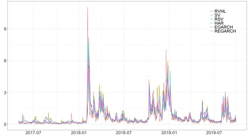
It is worth checking when the predictive ability differs, that is, when the volatility forecasts of some models are
worse than others. To this end, we present the cumulative loss for the volatility forecasts using MSE and QLIKE
in Figure 4. For both DJIA and N225, both MSE and QLIKE of the SV and EGARCH models gradually worsen
from the beginning of the prediction period, reflecting the results that the models using RV outperform the models
without RV.
For DJIA, the MSE shows notable leaps in early and late 2018. The leaps clearly coincide with rises in 5-minute
RV. After the surge of volatility in late 2018, the RSV model performs better than the HAR model and takes the
lowest MSE value among the models. On the other hand, the QLIKE shows small jumps in late 2017 and early
2018, making the volatility forecasts of the REGARCH model worse than the RSV and HAR models. After the
4 Specifically, we compute the adjustment term c for the RV at time t as follows:
∑t
s=t−n+1 (ys − ȳ)
2
1 ∑t
c= ∑t , ȳ = ys ,
s=t−n+1 RVs n s=t−n+1
where n denotes the fixed window size.
5 Following Takahashi et al. (2016), we use the constant and lagged loss differences as test functions.
14surge of volatility in early 2018, the RSV model outperform the HAR model and the difference of the MSE between
them gradually increases until the end. These results suggest that the differences of predictive ability are caused
by the rise of volatility.
For N225, the MSE also shows notable leaps in early and late 2018 and small jumps in late 2017, causing small
differences among the models using RV. After the surge of volatility in late 2018, the RSV model provides the lowest
MSE value. The QLIKE shows small jumps in late 2017 and early 2018. After the small jump in early 2018, the
RSV model performs best until the end. Although the differences among the models using RV are small, we argue
that the differences of predictive ability are partly due to the rise of volatility.
5 Conclusion
This paper compares the volatility predictive ability among the SV, RSV, HAR, EGARCH and REGARCH models
using daily return and RV of DJIA and N225. The RSV model gives the best predictive ability, measured by MSE
and QLIKE, for both DJIA and N225. Implementing the predictive ability test and undertaking an analysis based
on the model confidence set, we confirm that the models using RV outperform the models without RV. This suggests
that the RV provides the useful information on forecasting volatility. Overall, the RSV model performs best and
the HAR model can compete with it. The cumulative loss analysis suggests that the differences of the predictive
abilities among the models are partly caused by the rise of volatility.
Acknowledgement
Financial support from the Ministry of Education, Culture, Sports, Science and Technology of the Japanese Gov-
ernment through Grant-in-Aid for Scientific Research (No.16H036050 and 20H00073) and the Hitotsubashi Institute
for Advanced Study is gratefully acknowledged. All remaining errors are solely our responsibility.
Appendix
A Generation of h
Let αt = ht − µ, σϵ = exp(µ/2) and c = ξ + µ. The RSV model is now given by
yt = exp(αt /2)ϵ∗t , t = 1, . . . , n, (25)
xt = c + αt + ut , t = 1, . . . , n, (26)
αt+1 = ϕαt + ηt , t = 0, . . . , n − 1, (27)
15where
∗
ϵ
t σϵ2 ρσϵ ση 0
η ∼ N (0, Σ∗ ), Σ =
∗
ση2 0
t ρσϵ ση .
ut 0 0 σu2
The likelihood of (yt , xt ) given αt , αt+1 and other parameters excluding the constant term is
αt (yt − µt )2 (xt − c − αt )2
lt = − − − , (28)
2 2σt2 2σu2
where
ρσϵ σ −1 (αt+1 − ϕαt ) exp(αt /2),
η t = 1, . . . , n − 1,
µt = (29)
0, t = n,
(1 − ρ2 )σ 2 exp(αt ), t = 1, . . . , n − 1,
ϵ
σt2 = (30)
σϵ2 exp(αn ), t = n.
To sample α = (α1 , . . . , αn )′ from its conditional posterior distribution, we divide it into multiple blocks, and
generate one block, α(i) = (αs+1 , . . . , αs+m )′ , given other blocks. We sample η (i) = (ηs , . . . , ηs+m−1 )′ and then
obtain αt (t = s + 1, . . . , s + m) recursively, since it is known to be more efficient than sampling the state α(i) (e.g.
Durbin and Koopman (2002)). To sample η (i) , we conduct MH algorithm. We propose a candidate from normal
distribution which is obtained by the second order Taylor expansion of the log posterior density around the mode
η̂ (i) as below.
Define dt , At , Bt as
1 (yt − µt )2 yt − µt ∂µt yt−1 − µt−1 ∂µt−1 (xt − c − αt )
dt = − + + + + + κ(αt ),
2 2σt2 σt2 ∂αt 2
σt−1 ∂αt σu2
( )2 ( )2
1 ∂µt ∂µt−1 1
At = + σt−2 −2
+ σt−1 + 2 + κ′ (αt ),
2 ∂αt ∂αt σu
−2 ∂µt−1 ∂µt−1
Bt =σt−1 ,
∂αt−1 ∂αt
16where
{ } (α )
ρσϵ αt+1 − ϕαt
∂µt −ϕ + exp
t
, t < n,
= σ η 2 2 (31)
∂αt
0, t = n,
0, t = 1,
∂µt−1
= ρσ (α ) (32)
∂αt
ϵ
exp
t−1
, t > 1.
ση 2
ϕ(αt+1 − ϕαt )
, t=s+mwhere
Zt = 1 + Kt−1 Jt+1 ϕ, Gt = Kt−1 [1, Jt+1 ση ], Ht = [0, ση ].
Implement Kalman filter and the disturbance smoother to (35) and (36), and obtain the mode {ξ̂t }s+m−1
t=s of
the log conditional posterior density of {ξt }t=s
s+m−1
. Compute η̂t = Ht ξ̂t (t = s, . . . , s + m − 1) to obtain η̂ (i) ,
α̂(i) (e.g. Koopman (1993)).
6. Go to Step 2 until convergence. Usually, it is sufficient to repeat only a small number of times.
Next we conduct MH algorithm.
7. Let η (i) and η̂ (i) denote the current sample and the mode of the log posterior density.
8. Implement Steps 2–4 to update the linear Gaussian state space model (35)–(36). Let f ∗ (η (i) |·) denote the
conditional posterior density of η (i) (e.g. Takahashi et al. (2009)).
9. Propose a candidate using the simulation smoother (e.g. Omori and Watanabe (2008), deJong and Shephard
(1995), Durbin and Koopman (2002)) for the above linear and Gaussian state space model and accept it with
probability
{ }
f (η †(i) |·)f ∗ (η (i) |·)
min ,1
f (η (i) |·)f ∗ (η †(i) |·)
where f (η (i) |·) denotes the target log conditional posterior density. Alternatively, we may use
{ }
f˜(η (i) |·) ∝ min f (η (i) |·), c0 f ∗ (η (i) |·)
(c0 is some constant), and conduct the Acceptance-Rejection MH algorithm.
References
Aas, K. and Haff, I. H. (2006) The generalized hyperbolic skew Student’s t-distribution, Journal of Financial
Econometrics, 4, 275–309.
Abanto-Valle, C. A., Lachos, V. H. and Dey, D. K. (2015) Bayesian estimation of a skew-student-5 stochastic
volatility model, Methodology and Computing in Applied Probability, 17, 721–738.
Aı̈t-Sahalia, Y., Mykland, P. A. and Zhang, L. (2005) How often to sample a continuous-time process in the presence
of market microstructure noise, Review of Financial Studies, 18, 351–416.
Aı̈t-Sahalia, Y. and Mykland, P. A. (2009) Estimating volatility in the presence of market microstructure noise:
18A review of the theory and practical considerations, Andersen, T.G., Davis, R.A., Kreiß, J.-P. and Mikosch, T.
(eds), Handbook of Financial Time Series, 555–575, Berlin, Springer.
Andersen, T. G. and Benzoni, L. (2009) Realized volatility, Andersen, T. G., Davis, R. A., Kreiß, J.-P. and Mikosch,
T. (eds), Handbook of Financial Time Series, 555–575, Berlin, Springer.
Andersen, T. G., Bollerslev, T., Diebold, F. X., and Ebens, H. (2001a) The distribution of stock returns volatilities.
Journal of Financial Economics, 61, 43–76.
Andersen, T. G., Bollerslev, T., Diebold, F. X., and Labys, P. (2001b) The distribution of realized exchange rate
volatility, Journal of the American Statistical Association, 96, 42–55.
Andersen, T. G., Bollerslev, T., Diebold, F. X., and Labys, P. (2003) Modeling and forecasting realized volatility,
Econometrica, 71, 579–625.
Azzalini, A. and Capitanio, A. (2003) Distributions generated by perturbation of symmetry with emphasis on a
multivariate skew t-distribution, Journal of the Royal Statistical Society B, 65, 367–389.
Bandi, F. M. and Russell, J. R. (2006) Separating microstructure noise from volatility, Journal of Financial Eco-
nomics, 79, 655–692.
Bandi, F. M. and Russell, J. R. (2008) Microstructure noise, realized volatility, and optimal sampling, Review of
Economic Studies, 75, 339–369.
Barndorff-Nielsen, O. E., Hansen, P. R., Lunde, A., and Shephard, N. (2008) Designing realized kernels to measure
the ex-post variation of equity prices in the presence of noise, Econometrica, 76, 1481–1536.
Barndorff-Nielsen, O. E., Hansen, P. R., Lunde, A., and Shephard, N. (2009) Realized kernels in practice: Trades
and quotes, Econometrics Journal, 12, C1–C32.
Beran, J. (1994) Statistics for long-memory processes, Chapman & Hall.
Bollerslev, T. and Wooldridge (1992) Quasi maximum likelihood estimation and inference in dynamic models with
time varying covariances, Econometric Reviews, 11, 143–172.
Chib, S. (2001) Markov chain MOnte Carlo methods: computation and inference, Heckman, J.J. and Leamer E.
(eds.) Handbook of Econometrics, 3569–3649, Elsevier.
Corsi, F. (2009) A simple approximate long memory model of realized volatility, Journal Financial Econometrics,
7, 174–196.
de Jong, P. and Shephard, N. (1995) The simulation smoother for time series models, Journal of Royal Statistical
Society, Series B, 82, 339–350.
19Diebold, F. X. (1988) Empirical Modeling of Exchange Rate Dynamics, Springer-Verlag, Berlin.
Durbin, J. and Koopman, S. J. (2002) A simple and efficient simulation smoother for state space time series analysis,
Journal of Royal Statistical Society, Series B, 89, 603-616.
Giacomini, F. and White, H. (2006) Tests of conditional predictive ability, Econometrica, 74, 1545–1578.
Hansen, P. R. and Huang, Z. (2016) Exponential GARCH modeling with realized measures of volatility, Journal of
Business & Economic Statistics, 34, 269–87.
Hansen, P.R., Huang, Z., and Shek, H.H. (2012) Realized GARCH: a joint model for returns and realized measures
of volatility, Journal of Applied Econometrics, 27, 877–906.
Hansen, P. R. and Lunde, A. (2005) A forecast comparison of volatility models: Does anything beat a GARCH(1,1)?,
Journal of Applied Econometrics, 20, 873–889.
Hansen, P. R. and Lunde, A. (2006) Realized variance and market microstructure noise, Journal of Business &
Economic Statistics, 24, 127–161.
Hansen, P., Lunde, A. and Nason, J. (2011) The Model Confidence Set, Econometrica, 79, 453–497.
Jarque, C. M. and Bera, A. K. (1987) Test for normality of observations and regression residuals, International
Statistical Review, 55, 163–172.
Koopman, S. J. (1993) Disturbance smoother for state space models, Journal of Royal Statistical Society, Series B,
80, 117–126.
Koopman, S. J., Jungbacker, B. and Hol, E. (2005) Forecasting daily variability of the S&P 100 stock index using
historical, realized and implied volatility measurements, Journal of Empirical Finance, 12, 445–475.
Liu, L. Y., Patton, A. J. and Sheppard, K. (2015) Does anything beat 5-minute RV? A comparison of realized
measures across multiple asset classes, Journal of Econometrics, 187, 293–311.
Ljung, G. M. and Box, G. E. P. (1978) On a measure of lack of fit in time series analysis, Biometrika, 65, 297–303.
McAleer, M. and Medeiros, M.C. (2008) Realized volatility: a review, Econometric Reviews, 27, 10–45.
Nakajima, J. and Omori, Y. (2012) Stochastic volatility model with leverage and asymmetrically heavy-tailed error
using GH skew student’s t-distribution, Computational Statistics & Data Analysis, 56, 3690–3704.
Nelson, D. B. (1991) Conditional heteroskedasticity in asset returns: a new approach, Econometrica, 59, 347–370.
Newey, W. K. and West K. D. (1987) A simple positive semi-definite, heteroskedasticity and autocorrelation con-
sistent covariance matrix, Econometrica, 55, 703-708.
20Omori, Y., Chib, S., Shephard, N. and Nakajima, J. (2007). Stochastic volatility with leverage: fast likelihood
inference, Journal of Econometrics, 140, 425–229.
Omori, Y. and Watanabe, T. (2008) Block sampler and posterior mode estimation for asymmetric stochastic volatil-
ity models, Computational Statistics & Data Analysis, 52, 2892–2910.
Patton, J.A. (2011) Volatility forecast comparison using imperfect volatility proxies, Journal of Econometrics, 160,
246–256.
Takahashi, M., Omori, Y. and Watanabe, T. (2009) Estimating stochastic volatility models using daily returns and
realized volatility simultaneously, Computational Statistics & Data Analysis, 53, 2404–2426.
Takahashi, M., Watanabe, T. and Omori, Y. (2016) Volatility and Quantile Forecasts by Realized Stochastic
Volatility Models with Generalized Hyperbolic Distribution, International Journal of Forecasting, 32, 437–457.
Ubukata, M. and Watanabe, T. (2014) Option pricing using realized volatility, Japanese Economic Review, 65,
431–467.
Zhang, L. (2006) Efficient estimation of stochastic volatility using noisy observations: a multi-scale approach,
Bernoulli, 12, 1019–1043.
Zhang, L., Mykland, P. A. and Aı̈t-Sahalia, Y. (2005) A tale of two time scales: determining integrated volatility
with noisy high-frequency data, Journal of the American Statistical Association, 100, 1394–1411.
21Table 1: Descriptive statistics of the daily returns and logarithms of the 5-minute RVs.
DJIA Mean SD Skew Kurt Min Max JB LB
Daily Return 0.000 0.009 -0.447 6.675 -0.056 0.049 0.000 0.522
Log RV -10.197 1.048 0.317 3.175 -13.163 -5.123 0.000 0.000
N225 Mean SD Skew Kurt Min Max JB LB
Daily Return 0.000 0.013 -0.544 8.101 -0.112 0.074 0.000 0.554
Log RV -10.068 0.844 0.588 4.219 -12.531 -5.953 0.000 0.000
The time periods covered are from June 1, 2009 to September 27, 2019, for DJIA (2,596 samples), and from
June 1, 2009 to September 30, 2019, for N225 (2,532 samples). The DJIA data are obtained from Oxford-Man
Institute’s “realized library” and the N225 data are constructed from Nikkei NEEDS-TICK dataset. Standard
errors of skewness and kurtosis are 0.048 and 0.096, respectively, for DJIA, whereas those for Nikkei 225 are 0.049
and 0.097, respectively. JB is the p-value of the Jarque-Bera statistic for testing the null hypothesis of normality.
LB is the p-value of the Ljung and Box (1978) statistic adjusted for heteroskedasticity following Diebold (1988) to
test the null hypothesis of no autocorrelation up to 10 lags.
Table 2: MCMC estimation results of SV and RSV models for the first rolling window.
DJIA N225
Parameter SV RSV SV RSV
ϕ 0.9391 (0.0097) 0.9244 (0.0101) 0.9202 (0.0168) 0.8989 (0.0130)
[0.9185, 0.9568] [0.9038, 0.9430] [0.8828, 0.9482] [0.8717, 0.9231
94.88 33.20 123.81 26.00
ση 0.3259 (0.0097) 0.3121 (0.0179) 0.2977 (0.0371) 0.3003 (0.0167)
[0.2712, 0.3910] [0.2788, 0.3487] [0.2330, 0.3737] [0.2691, 0.3353]
172.16 65.51 193.99 24.42
ρ −0.7354 (0.0456) −0.5378 (0.0384) −0.6075 (0.0526) −0.3945 (0.0759)
[−0.8113, −0.6365] [−0.6108, −0.4608] [−0.7014, −0.4968] [−0.3565, −0.1952]
87.68 35.91 38.83 24.42
µ −0.4137 (0.0972) −0.5102 (0.0903) 0.4528 (0.0803) 0.3945 (0.0759)
[−0.5986, −0.2153] [−0.6857, −0.3286] [0.2984, 0.6143] [0.2482, 0.5464]
4.48 6.44 4.77 12.41
ξ −0.1897 (0.0411) −1.0706 (0.0382)
[−0.2732, −0.1125] [−1.1472, −0.9974]
19.92 39.75
σu 0.5295 (0.0131) 0.3996 (0.0129)
[0.5041, 0.5552] [0.3738, 0.4248]
24.56 35.25
The sample period is from June 1, 2009, to April 28, 2017, for both DJIA and N225, corresponding to the first
window estimation with the fixed window size 1,993 and 1,942, respectively. The results are obtained using 15,000
samples recorded after discarding 5,000 samples from MCMC iterations. The latent volatility h for both SV and
RSV models are sampled via using the block sampler. The first row presents the posterior mean with the standard
deviation in the parenthesis. The the second and third rows are the 95% credible interval and the inefficiency
factor by Chib (2001). The priors are set as µ ∼ N (0, 100), (ϕ + 1)/2 ∼ Beta(20, 1.5), (ρ + 1)/2 ∼ Beta(1, 2),
ση2 ∼ IG(2.5, 0.025), ξ ∼ N (0, 1), and σu2 ∼ IG(2.5, 0.1).
22Table 3: Ordinary least squares (OLS) estimation results of HAR model for the first rolling window.
Parameter DJIA N225
β0 −0.3544 (0.0271) −0.2693 (0.0208)
βd 0.2026 (0.0375) 0.1789 (0.0337)
βw 0.3832 (0.0457) 0.2841 (0.0465)
βm 0.2291 (0.0349) 0.3443 (0.0340)
λ −0.2641 (0.0342) −0.1310 (0.0176)
Adjusted R2 0.5282 0.5453
The sample period is from June 1, 2009, to April 28, 2017, for both DJIA and N225, corresponding to the first
window estimation with the fixed window size 1,993 and 1,942, respectively. The table shows the OLS estimates
and the adjusted R2 with the Newey-West standard errors allowing for serial correlation of up to order 5 in the
parentheses.
Table 4: Quasi-maximum likelihood (QML) estimation results of EGARCH and REGARCH models for the first
rolling window.
DJIA N225
Parameter EGARCH REGARCH EGARCH REGARCH
ω −0.2464 (0.0866) −0.4140 (0.0792) −0.2362 (0.0866) 0.5161 (0.0908)
φ 0.9412 (0.0103) 0.9381 (0.0082) 0.9402 (0.0101) 0.9192 (0.0140)
τ −0.2028 (0.0214) −0.2092 (0.0215)
τ1 −0.1805 (0.0123) −0.1104 (0.0119)
τ2 0.0384 (0.0070) 0.0612 (0.0100)
γ 0.1608 (0.0232) 0.2305 (0.0208) 0.1630 (0.0234) 0.3121 (0.0315)
ζ −0.3118 (0.0353) −1.2147 (0.0440)
δ1 −0.1145 (0.0142) −0.1239 (0.0118)
δ2 0.1630 (0.0134) 0.0970 (0.0089)
σu2 0.3281 (0.0116) 0.2290 (0.0107)
The sample period is from June 1, 2009, to April 28, 2017, for both DJIA and N225, corresponding to the first
window estimation with the fixed window size 1,993 and 1,942, respectively. The table shows the quasi-maximum
likelihood estimates with the QML robust standard errors in the parentheses. correction .
Table 5: Mean squared error (MSE) and quasi-likelihood (QLIKE) of volatility forecasts for DJIA and N225.
DJIA N225
MSE QLIKE MSE QLIKE
SV 0.541 0.287 1.224 0.233
RSV 0.416 0.188 1.105 0.162
HAR 0.419 0.197 1.161 0.165
EGARCH 0.454 0.290 1.160 0.219
REGARCH 0.425 0.212 1.151 0.171
The MSE and QLIKE are calculated from the 603 prediction samples from 603 prediction samples from May 1,
2017, to September 27, 2019, for DJIA, and 590 prediction samples from May 1, 2017, to September 30, 2019, for
N225. The 5-minute RV with the adjustment of Hansen and Lunde (2005) is used as a proxy for the latent volatility.
23Table 6: The results of the predictive ability test of Giacomini and White (2006).
DJIA
SV RSV HAR EGARCH REGARCH
SV – 0.000 0.000 0.238 0.000
RSV 0.010 – 0.303 0.000 0.156
HAR 0.172 0.705 – 0.000 0.300
EGARCH 0.001 0.210 0.767 – 0.000
REGARCH 0.028 0.432 0.396 0.381 –
N225
SV RSV HAR EGARCH REGARCH
SV – 0.000 0.000 0.011 0.000
RSV 0.070 – 0.487 0.000 0.000
HAR 0.176 0.865 – 0.000 0.187
EGARCH 0.101 0.502 0.512 – 0.000
REGARCH 0.518 0.000 0.176 0.156 –
The numbers indicates the p-values of the test statistics with the null of equal predictive ability of the pair of
models. The lower and upper triangular parts represent the p-values for MSE and QLIKE, respectively.
Table 7: The results of 90% model confidence set (MCS) of Hansen et al. (2011).
DJIA N225
MSE QLIKE MSE QLIKE
SV – – 0.320 –
RSV 1.000 1.000 1.000 1.000
HAR 1.000 1.000 1.000 0.244
EGARCH 0.378 – 1.000 –
REGARCH 1.000 0.121 1.000 –
The models with numbers are in the 90% MCS. The numbers show the MCS p-values for MSE and QLIKE of
volatility forecasts. The results are obtained by implementing R package MCS using Tmax as the test statistic with
1,000 bootstrap replications and block size equal to 10.
24You can also read