A PROBABILISTIC APPROACH TO IDENTIFYING RUN SCORING ADVANTAGE IN THE ORDER OF PLAYING CRICKET
←
→
Page content transcription
If your browser does not render page correctly, please read the page content below
A P ROBABILISTIC A PPROACH TO I DENTIFYING RUN S CORING
                                                    A DVANTAGE IN THE O RDER OF P LAYING C RICKET

                                                                   Manar D. Samad                                     Sumen Sen
                                                            Department of Computer Science              Department of Mathematics and Statistics
                                                              Tennessee State University                      Austin Peay State University
                                                                  Nashville, TN, USA                            Clarksville, TN, USA
arXiv:2007.05894v1 [stat.AP] 12 Jul 2020

                                                                msamad@tnstate.edu

                                                                                                 July 14, 2020

                                                                                                A BSTRACT
                                                    In the game of cricket, the result of coin toss is assumed to be one of the determinants of match
                                                    outcome. The decision to bat first after winning the toss is often taken to make the best use of superior
                                                    pitch conditions and set a big target for the opponent. However, the opponent may fail to show their
                                                    natural batting performance in the second innings due to a number of factors, including deteriorated
                                                    pitch conditions and excessive pressure of chasing a high target score. The advantage of batting
                                                    first has been highlighted in the literature and expert opinions, however, the effect of batting and
                                                    bowling order on match outcome has not been investigated well enough to recommend a solution
                                                    to any potential bias. This study proposes a probability theory-based model to study venue-specific
                                                    scoring and chasing characteristics of teams under different match outcomes. A total of 1117 one-day
                                                    international matches held in ten popular venues are analyzed to show substantially high scoring
                                                    advantage and likelihood when the winning team bat in the first innings. Results suggest that the
                                                    same ‘bat-first’ winning team is very unlikely to score or chase such a high score if they were to
                                                    bat in the second innings. Therefore, the coin toss decision may favor one team over the other. A
                                                    Bayesian model is proposed to revise the target score for each venue such that the winning and scoring
                                                    likelihood is equal regardless of the toss decision. The data and source codes have been shared
                                                    publicly for future research in creating competitive match outcomes by eliminating the advantage of
                                                    batting order in run scoring.

                                           Keywords Coin toss; Cricket; Bayesian rule; Batting order; Negative binomial distribution; Sports analytics; One-day
                                           international

                                           1    Introduction
                                           The game of cricket has more than two billion fans and followers over the world with 104 cricket playing nations.
                                           One-day international (ODI) and T-20 formats are the most popular versions of cricket that are played between teams in
                                           home-away series, world-cup tournaments, and domestically at first class tournaments and premium leagues. In the
                                           game of cricket, one team (Team A) bat first (first innings) to score ’runs’ by competing against the bowling and fielding
                                           performance of the opponent team (Team B). In ODI, eleven players (ten wickets) of team A bat in the first innings to
                                           score a total ‘run’ facing 50 overs (300 balls, 6 balls per over) of bowling delivery of the opponent team B. Following
                                           a half-time break, the team B bat in the second innings to chase the target score playing against 50 overs of bowling
                                           delivery of team A. Team A win, tie, or lose the match if team B score less, equal, or more than the first innings target
                                           score set by Team A, respectively. The same strategy is followed in the T-20 version of the game, but each team is given
                                           only 20 overs (120 balls) to score or chase instead of 50 overs.
                                           Unlike other popular sports such as soccer, hockey, basketball, the game of cricket is unique that involves heavy
                                           accounting and diverse statistics to evaluate or predict the performance of a team or individual players. Statistical
                                           analyses may play a valuable role in determining an effective game strategy and team selection [3] , analyzing outcome
A PREPRINT - J ULY 14, 2020
0.008 1.0 1.0
PDF CDF 1-CDF
0.007
0.006 0.8 0.8
0.005
Probability
Probability
Probability
0.6 0.6
0.004
0.003 0.4 0.4
0.002
0.2 0.2
0.001
0.000 0.0 0.0
0 100 200 300 400 0 100 200 300 400 0 100 200 300 400
Score in runs Score in runs Score in runs
(a) (b) (c)
Figure 1: (a) Probability density function, P(x), (b) cumulative density function (CDF) of P(X), and (c) complement of
CDF of scoring runs representing probability of scoring greater than X runs.
in the second innings based on target set in the first innings [6] , assessing the performance of players [2] , ordering of
eleven players during the batting session [21] , and predicting outcome of a match [1,4] .
Therefore, historical data obtained from thousands of ODI cricket matches along with data-driven statistical methods
can be valuable resources for operational research and management, performance evaluation, updating game rules, and
forecasting results [15] . One of the most popular statistical models adopted in Cricket is the Duckworth-Lewis (DL)
method that determines a revised and fair target score when the game is interrupted, and the match duration is shortened
by rain [9] . In the past, the event of rain not only postponed the match, but also unfairly penalized one of the teams by
cutting their allotted overs for batting. The DL method has been used for over two decades to set a reasonable target by
statistically considering partial match results and resources (wickets and overs) available prior to the rain. This method
has been an active subject of research and modification over the last two decades [13,18] .
Apart from rain interrupted events, there are numerous implicit sources of bias that may unfairly favor one team over
another [10] . For example, the home ground advantage is inevitable that is likely to favor the hosting team in a cricket
match [16] . The innings played at night time in a day-night match has shown considerable difference in outcome when
compared to its counterpart innings played in the day time [12] . One of the debated issues in Cricket is the decision
whether a team should bat or bowl first following a toss of a fair coin. This decision has been argued to give an
advantage to the toss winning team. Sood and Willis have shown in a recent study that the winning of coin toss has
a significant effect on winning the game, especially when the contesting teams have matching performance, and the
match is played in certain conditions such as in the day-night format [20] . In general, a team choose to bat first expecting
to set a high scoring target using superior field conditions in the first half of the match. The pitch condition is expected
to deteriorate over time, which may eventually turn less favorable for batting in the second innings. In contrast to this
thought, the decision to bat first is also perturbed by a concern that a ‘safe’ score for confirming victory is unknown
while batting in the first innings. Therefore, a team may choose to bowl first as they prefer to have a ‘known’ target
score to chase expecting that field conditions or weather may rather turn unfavorable to bowlers in the second innings.
Eventually, the coin toss decision inevitably tends to favor one team over another to some extent, which may not always
give both teams a fair chance to win the match. Furthermore, statistics from the last four world cup cricket tournaments
suggest that the teams winning the toss and deciding to bowl first are victorious in less than 50% of similar cases [7] .
This phenomenon reveals certain advantages in batting first over bowling apparently due to a number of confounding
factors. In support to this observation, Dawson et al. have concluded in their study that winning the toss and batting
first significantly increases the chance of winning the match compared to the decision of bowling first after winning the
toss [8] .
1.1 Proposed research
In line with above observations, we identify two cases that may significantly bias the outcome of the game due to coin
toss-based decision of batting or bowling order. First, it is widely known that chasing a target score of over 300 runs in
the second innings is often more challenging than scoring such high total in the first innings. This becomes more true
even while chasing a decent target in the fourth innings of Test cricket. For example, there are only nine matches in over
forty years of world cup cricket history where the bat-second team have been able to chase a target score of 300 and
above runs. However, there are at least 19 matches in the 2019 world cup alone where the first innings scores are more
than 300. Therefore, deciding to bat first and setting a big target appears to lower the probability of successfully chasing
the target in the second innings even with two equally competitive teams. Second, first innings batting experience is
2A PREPRINT - J ULY 14, 2020
free of pressure from chasing a target score, which is a psychological advantage. The team batting in the second innings
incur this additional pressure and such pressure may negatively affect their natural batting performance. Even a very
competitive team have been seen to collapse by scoring unusually low score while chasing an unusually high score [5] ,
which is often termed as ’choking’ or ‘strangling’ and has been studied by Lemmer [11] . All these phenomena do not
guarantee equal opportunity for teams to compete in a fair ground since the coin toss decision may ultimately influence
the outcome of the game. These issues can negatively affect the excitement, competitiveness, and spirit of the game.
All these statistics raise a number of research questions that demand data-driven solutions. First, is there any run scoring
advantage in the first innings score that might affect the outcome of the game? Second, what would the team score if
they were to bat in the second innings given the fact that they have scored a big and ‘hard-to-chase’ total in the first
innings? Third, what would be a reasonable and competitive target that accounts for the advantage of winning the
toss and setting an unusually high first innings score? Since there is apparently no alternative to coin tossing, we have
used probability theory on venue-specific ODI match results to investigate bias in run scoring distributions at different
playing conditions and match outcomes. A statistical model has been proposed to incorporate such venue-specific bias
for two purposes: 1) data mining to identify the magnitude of the bias and 2) recommending a revised target that will
equalize the probability of winning a big scoring match regardless of the playing order (bat first versus bowl first).
2 Methodology
This study proposes a probability-based model in investigating potential scoring bias following the decision of playing
order taken by tossing a coin. First, the scoring probability distributions of four match cases are obtained and compared
for each of ten ODI venues. The four match cases are: 1) bat-first-win, 2) bat-first-lose, 3) bat-second-win, 4) bat-
second-lose. The run distributions are modeled using negative binomial (NB) distribution since it effectively represents
run distributions in Scarf et al. [19] . The NB distribution modeling a discrete random variable x is shown as below.
Γ(x + n) n
P (x, n, p) = p (1 − p)x . (1)
Γ(n)x!
The parameters of NB distribution (n and p) are obtained using maximum likelihood estimates to yield the probability
mass function (PMF). For comparison, probability density function (PDF) of contribution variable distributions are
developed using mean and variance of the scores. The PMF or PDF represent the scoring probability distribution, P(X).
Figure 1(a) shows the PDF of a normal distribution. Intuitively the probability of scoring a total of exactly Xt runs P(X
= Xt) (e.g. 237 runs) is low when the sample space is large typically ranging from 100 runs to 350 runs. Intuitively,
scoring a total of 200 runs and more is much higher than scoring 300 runs and more. This leads to the definition of
cumulative PDF that represents the probability of scoring up to Xt runs, P (X≤Xt) by integrating or summing the PDF
or PMF from zero to Xt, respectively as shown in Figure 1(b). We take complement of CDF in Eq. 1 to represent our
intuition that scoring at least 200 runs P(X>200) is higher than that of scoring at least 300 runs, P(X>300), as shown in
Figure 1(c).
x=xt
X
P (X > Xt) = 1 − P (X ≤ Xt) = 1˘ P (x, n, p) (2)
x=0
where, P(X,n,p) is the best fitted PMF on the data. We use the complement of CDF in subsequent comparisons among
four match cases to investigate bias in scoring probability.
2.1 Bayesian model
In the presence of a scoring bias, we propose a Bayesian model to recommend a revised target score that will equalize
the scoring and winning probability of both innings irrespective of the coin toss decision. First, the variables and
outcomes are identified for ODI cricket matches. The match outcome can be either win (W) or lose (L). First and
second innings batting conditions are represented by BF and BS, respectively. We define the posterior probability of
winning a match given that the team bat first and score at least Xf runs in the first innings as P (W | S>Xf, BF). Using
the Bayes’ rule, this posterior winning probability can be calculated as below.
P (S > Xf, BF | W ) P (W )
P (W | S > Xf, BF ) = (3)
P (S > Xf, BF )
3A PREPRINT - J ULY 14, 2020
Similarly, the posterior probability of winning the match given that the winning team bat in the second innings and
score Xs runs is as follows.
P (S > Xs, BS | W ) P (W )
P (W | S > Xs, BS) = (4)
P (S > Xs, BS)
Given a first innings score of at least Xf runs, the minimum second innings target score Xs that will equalize the winning
probability of any team in a particular venue is obtained by equalizing Eqs. 3 and 4 as below.
P (S > Xs, BS | W ) P (S > Xf, BF | W )
= (5)
P (S > Xs, BS) P (S > Xf, BF )
Applying the chain rule of conditional probability,
P (S > Xs | BS, W ) P (BS | W ) P (S > Xf | BF, W ) P (BF | W )
= (6)
P (S > Xs, BS) P (S > Xf, BF )
Joint probability distributions in the denominator can be expressed in terms of conditional probability distributions.
P (S > Xs | BS, W ) P (BS | W ) P (S > Xf | BF, W ) P (BF | W )
= (7)
P (S > Xs | BS) P (BS) P (S > Xf | BF ) P (BF )
P (S > Xs | BS) P (BF | W )
P (S > Xs | BS, W ) = P (S > Xf | BF, W ). (8)
P (S > Xf | BF ) P (BS | W )
Here, the probability of batting first or second is equal, P(BF) = P(BS), considering the coin is fair. Given the first
innings score Xs, we assume that the revised second innings score Xf will additionally equalize the scoring probability
(in addition to the winning probability) of both innings such that P (S>Xf | BF)= P (S>Xs | BS). The revised equation
is as follows.
P (S > Xs | BS, W ) = C ∗ P (S > Xf | BF, W ) (9)
(Bf |W )
Here, C = PP (BS|W ) is a constant ratio for a venue, which is the ratio of probabilities of batting first and second given
that the team is victorious. In the case of higher likelihood of batting first of the winning team, the ratio will be greater
than 1. Given the first innings score Xf, the second innings score Xs that satisfies the two conditions can be obtained by
taking inverse of the CDF, P(S≤Xs|BS,W) as below.
Xs = Inv (P (S ≤ Xs | BS, W ))
= Inv (1 − C ∗ P (S > Xf | BF, W )) (10)
3 Results and Discussion
We have implemented the entire model in Python programming language using the scipy, numpy, and pandas pack-
ages [14,17] and shared the source codes, data, and notebook in a github repository. Results of all ODI matches are
obtained from the webpage of Cricket-stats 1 for ten most popular international venues as summarized in Table 1.
Table 1 shows that the bat-first-lose teams have higher average score than that of bat-second-lose teams.
3.1 Analysis of probability distributions
The probability distribution of run scored at each venue is studied by fitting the negative binomial distribution. The
NB distribution is one of the popular choices for modeling count data like runs in Cricket. The NB distribution is
also fitted to yield the overall distribution of runs regardless of the venue. The effect of batting and bowling order on
scoring distribution is analyzed by categorizing the distributions into four cases: 1) bat-first-win, 2) bat-second-lose, 3)
bat-first-lose, and 4) bat-second-win. Figure 2 shows scoring distributions of four experimental cases after fitting with
NB distribution using all venue data. Following this result, we assume that venue-specific distributions also follow the
NB distribution.
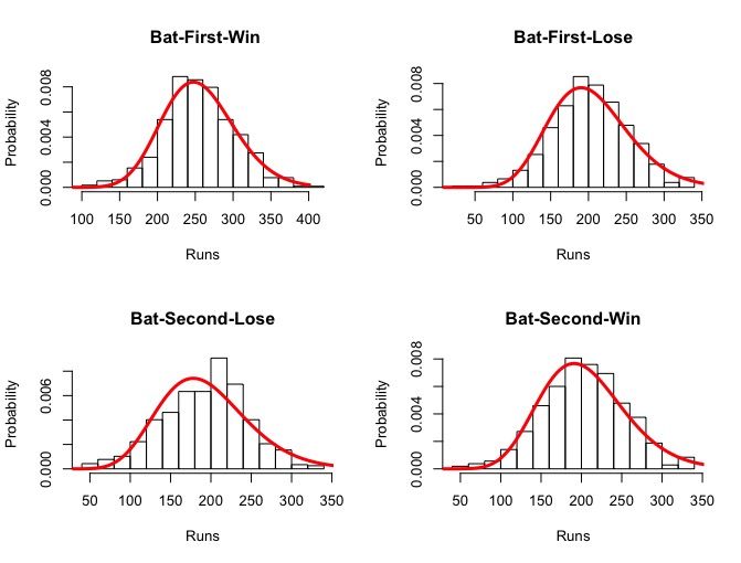
Figure 3 shows that the run distributions of bat-first-lose and bat-second-win are similar and overlapping for all venues.
This is intuitive since the bat-second-win team will always score one or several runs more than the bat-first-lose team.
1
http://cricket-stats.net/genp/grounds.shtml
4A PREPRINT - J ULY 14, 2020
Figure 2: Fitting runs of four experimental cases using the negative binomial distribution.
Table 1: Summary of one-day international cricket match results used in this study. Average runs are rounded off to the
next integer value. Since Bat-second-win teams score as much as Bat-first-lose teams, their run scoring distributions
appear similar.
Venue Total match Bat-first-win Bat-second-lose Bat-second-win Bat-first-lose
% Avg. score Avg. score % Avg. score Avg. score
Auckland 71 42.3 240 185 57.7 200 203
Bangalore 22 50.0 294 248 50.0 236 234
Harare 149 49.7 255 183 50.3 205 204
Lahore 58 56.9 266 205 43.1 233 231
Lords 62 48.4 268 215 51.6 218 217
Melbourne 145 49.7 245 191 50.3 202 201
Mirpur 107 46.7 261 194 53.3 203 204
Premadasa 118 58.5 266 196 41.5 204 203
Sharjah 236 53.8 252 189 46.2 195 192
Sydney 149 59.1 248 189 40.9 195 198
Overall 1117 51.5 260 200 48.5 209 209
These two cases have yielded same average score of 209 runs over 1117 ODI matches (Table 1). However, the scoring
distribution of bat-second-lose teams falls behind that of bat-first-lose teams for almost all venues. That is, batting first
yields higher scoring probability than that of batting in the second innings even when both cases the team lose the
match. This discrepancy is indicative of a scoring bias or advantage possibly due to the batting order. This advantage
in run scoring is more evident at venues like Premadasa, Harare, Lahore and lowest at Sharjah, Sydney, and Lords.
The only exception is the venue at Bangalore where the bat-second-lose scoring probability is better than that of the
bat-first-lose case. This observation may be attributed to the lowest sample size for Bangalore (only 22 ODI matches
grouped into four categories) compared to other venues (Table 1).
However, this is not the case when the bat-first team win the match against the bat-second-lose team. The data reveal
that the ’bat-second-lose’ teams have the worst scoring performance and their opponent ’bat-first-win’ teams have the
best scoring distribution among all four cases. The scoring distribution of bat-first-win teams is far ahead of those of
other three cases for all venues (Figure 3). This distribution also infers that the same high scoring team in the first
innings is likely to score lower in the second innings. This suggests an extra disadvantage of batting in the second
5A PREPRINT - J ULY 14, 2020
Auckland Lords
1.0 Bat First Win 1.0 Bat First Win
Bat Second Lose Bat Second Lose
0.8 Bat Second Win 0.8 Bat Second Win
Bat First Lose Bat First Lose
Probability
Probability
0.6 0.6
0.4 0.4
0.2 0.2
0.0 0.0
0 50 100 150 200 250 300 350 400 0 50 100 150 200 250 300 350 400
Score in runs Score in runs
Mirpur Premadasa
1.0 Bat First Win 1.0 Bat First Win
Bat Second Lose Bat Second Lose
0.8 Bat Second Win 0.8 Bat Second Win
Bat First Lose Bat First Lose
Probability
Probability
0.6 0.6
0.4 0.4
0.2 0.2
0.0 0.0
0 50 100 150 200 250 300 350 400 0 50 100 150 200 250 300 350 400
Score in runs Score in runs
Harare Bangalore
1.0 Bat First Win 1.0
Bat Second Lose
0.8 Bat Second Win 0.8
Bat First Lose
Probability
Probability
0.6 0.6
0.4 0.4
Bat First Win
0.2 0.2 Bat Second Lose
Bat Second Win
0.0 0.0 Bat First Lose
0 50 100 150 200 250 300 350 400 0 50 100 150 200 250 300 350 400
Score in runs Score in runs
Sydney Lahore
1.0 Bat First Win 1.0 Bat First Win
Bat Second Lose Bat Second Lose
0.8 Bat Second Win 0.8 Bat Second Win
Bat First Lose Bat First Lose
Probability
Probability
0.6 0.6
0.4 0.4
0.2 0.2
0.0 0.0
0 50 100 150 200 250 300 350 400 0 50 100 150 200 250 300 350 400
Score in runs Score in runs
Sharjah Melbourne
1.0 Bat First Win 1.0 Bat First Win
Bat Second Lose Bat Second Lose
0.8 Bat Second Win 0.8 Bat Second Win
Bat First Lose Bat First Lose
Probability
Probability
0.6 0.6
0.4 0.4
0.2 0.2
0.0 0.0
0 50 100 150 200 250 300 350 400 0 50 100 150 200 250 300 350 400
Score in runs Score in runs
Figure 3: Complement of cumulative negative binomial distribution of four cases: two playing orders (Bat first,
Bat Second) and two outcomes (win, lose) at ten ODI venues. All venues show large discrepancy between scoring
probabilities of ’bat-first-win’ teams and their opponent ’bat-second-lose’ teams.
6A PREPRINT - J ULY 14, 2020
Table 2: Revised second innings target score against a first-innings score (actual score). The revised scores are shown
for binomial distribution. The sum of difference between actual and revised scores are shown for the three distributions:
negative binomial, normal, and logistic. The overall model included data from all 1117 ODI matches and is not mere
aggregation of ten venue results.
Actual Target 300 315 330 340 350 Total difference in runs
Venue Negative binomial distribution Negative binomial Normal Logistic
Auckland 283 301 320 332 345 54 63 6
Bangalore 241 251 261 268 275 335 329 327
Harare 276 289 312 327 342 95 155 152
Lahore 251 266 280 289 298 250 233 283
Lords 263 284 306 321 335 120 145 134
Melbourne 267 286 304 317 329 131 164 163
Mirpur 255 273 291 303 316 197 211 184
Premadasa 225 243 260 271 282 355 363 420
Sharjah 242 259 277 289 301 267 282 308
Sydney 230 247 263 274 285 336 343 414
Overall model 249 266 284 295 307 234 245 261
innings to chase a large target set by the bat-first team. It is noteworthy that these discrepancies are venue-specific under
the assumption that stronger and weaker teams have similar likelihood of winning the toss or batting in the first innings.
Such discrepancies can be even more striking when the stronger side gets the chance to bat first and sets a large and
unattainable target to chase. Therefore, it is worth determining the total runs that the bat-first-win team would have
scored if they were sent to bat in the second innings. This revised score may inform us about the extent of bias and
recommend a fair target to be chased in the second innings to alleviate the effect of coin toss on match outcome.
3.2 Probabilistic model for revising target
The previous section reveals higher scoring probability of bat-first-win teams compared to that of any other three cases.
This high scoring probability can yield a target score that becomes very challenging to chase while batting in the second
innings. For example, the world cup record of chasing the highest score is 329 runs whereas first innings score has been
as high as 397 runs. There are at least eight matches in the 2019 cricket world cup alone with over 330 runs scored
in the first innings, which would require the opponent to break the world cup record to win those matches. Statistics
suggest that there are only a handful cases in the world cup cricket when a score of 300 runs and above is successfully
chased in the second innings. Therefore, after observing a very high score in the first innings, the game is assumed
over even before playing the second innings of the match. Commentary is made highlighting that there is no record of
chasing such a high score in this particular venue. These observations go against the ’glorious uncertainties’ of the
game of cricket.
One naive way to tackle this bias is to equalize the opportunity for both teams in a big scoring match by revising an
unusually big target score set in the first innings considering a venue-specific or overall probabilistic model. In this
study, we assume that any score over 300 runs is typically a tough score to chase in the second innings. A revised
target score for the second innings may be obtained using Eq. 10 that equalizes both winning and scoring probability of
the competing teams. Table 2 shows revised scores for a set of first innings scores over 300 runs using the proposed
probabilistic model. The revised scores obtained from the normal and logistic probability distribution are not too
different from those obtained from the negative binomial distribution. The total run difference between the actual target
(first innings score) and the model revised target is also a measure of bias for each venue. Results suggest that the venue
in Auckland has the lowest difference and the one in Premadasa has the highest differences for all three distribution
models. The negative binomial distribution has yielded the lowest differences in scoring among the three distributions
because it is known to best fit run scoring data. The last row of Table 2 shows the overall model results obtained after
fitting all 1117 match results from all ten venues. In all cases, the revised target score for the second innings team is
lower than that of the first innings score.
3.3 Limitations
The goal of this study is to investigate run scoring advantages due to batting in the first innings of cricket. The proposed
Bayesian model makes two assumptions to determine the revised score to alleviate the bias present in the first innings
7A PREPRINT - J ULY 14, 2020
score. The model equalizes both winning and scoring probabilities of a first innings score with those of a revised
second innings score. However, the assumption of equal winning probability, when the scoring probability is considered
unequal (P(S>Xf | BF) 6= P(S>Xs | BS)), complicates the solution and does not yield a robust solution of the revised
score. A more conservative estimate of the revised target (closer to the first innings score) may be obtained by relaxing
one of the two assumptions. Our model needs further search for robust solutions in providing more unbiased target
scores by relaxing one of the two model assumptions. A number of venues have comparatively low sample size, which
is further reduced due to grouping of the samples into four match cases. Therefore, venue-specific models may not be
reliable when the sample size is low. Conversely, there may be high variance in the model that includes all venue data.
The proposed model is not directly applicable for new venues unless past data are combined from all other existing
venues in the model development. There are no gold standard and benchmark data to evaluate the performance of the
proposed model because of its empirical nature.
4 Conclusions
This study has investigated run scoring distributions of different playing orders and outcomes in the one-day international
cricket. Our data clearly suggest an extra advantage of batting first in high scoring matches regardless of venues
and strength of the playing teams. The high scoring distribution of all bat-first-win cases also infers that the same
bat-first-win team is highly likely to score less if they were sent to bat in the second innings to chase the same score.
Our proposed Bayesian model has captured venue-specific run scoring distributions to show the magnitude of advantage
in the first innings batting for the winning team and to estimate revised target scores for the second innings. The revised
target scores ensure equal winning and scoring probability for a particular venue. Despite limitations in numerical
computations, we believe that this is one of the first studies to investigate such bias in the game of cricket with a
recommended solution. The proposed model can be used to investigate ordering bias in other research and operations to
subsequently recommend a revision to alleviate effects of any factor biasing the outcome.
References
[1] Sohail Akhtar and Philip Scarf. Forecasting test cricket match outcomes in play. International Journal of
Forecasting, 28(3):632–643, jul 2012. ISSN 0169-2070. doi: 10.1016/J.IJFORECAST.2011.08.005. URL
https://www.sciencedirect.com/science/article/pii/S0169207011001622.
[2] Sohail Akhtar, Philip Scarf, and Zahid Rasool. Rating players in test match cricket. Journal of the Operational
Research Society, 66(4):684–695, apr 2015. ISSN 0160-5682. doi: 10.1057/jors.2014.30. URL https://www.
tandfonline.com/doi/full/10.1057/jors.2014.30.
[3] Gholam R. Amin and Sujeet kumar Sharma. Cricket team selection using data envelopment analysis. European
Journal of Sport Science, 14(sup1):S369–S376, jan 2014. ISSN 1746-1391. doi: 10.1080/17461391.2012.705333.
[4] M. Asif and I.G. McHale. A generalized non-linear forecasting model for limited overs international cricket.
International Journal of Forecasting, 35(2):634–640, apr 2019. ISSN 0169-2070. doi: 10.1016/J.IJFORECAST.
2018.12.003. URL https://www.sciencedirect.com/science/article/pii/S0169207019300068.
[5] Dibyojyoti Bhattacharjee and Hermanus H Lemmer. Quantifying the pressure on the teams batting or bowling in
the second innings of limited overs cricket matches. International Journal of Sports Science & Coaching, 11(5):
683–692, oct 2016. ISSN 1747-9541. doi: 10.1177/1747954116667106. URL http://journals.sagepub.
com/doi/10.1177/1747954116667106.
[6] Dipankar Bose and Soumyakanti Chakraborty. Managing In-play Run Chases in Limited Overs Cricket Using
Optimized CUSUM Charts. Journal of Sports Analytics, 5(4):335–346, aug 2019. ISSN 2215020X. doi:
10.3233/jsa-190342. URL http://cricsheet.org/.
[7] Vaidik Dalal. The first innings conundrum in world cup 2019. URL https://www.livemint.com/sports/
cricket-news/the-first-innings-conundrum-in-world-cup-2019-1561614800105.html. [Online;
posted 27-June-2019].
[8] P. Dawson, B. Morley, D. Paton, and D. Thomas. To Bat or Not to Bat: An Examination of Match Outcomes in
Day-Night Limited Overs Cricket, 2009.
[9] F C Duckworth and A J Lewis. A fair method for resetting the target in interrupted one-day cricket matches.
Journal of the Operational Research Society, 49(3):220–227, mar 1998. ISSN 0160-5682. doi: 10.1057/palgrave.
jors.2600524. URL https://www.tandfonline.com/doi/full/10.1057/palgrave.jors.2600524.
8A PREPRINT - J ULY 14, 2020
[10] David Forrest and Ron Dorsey. Effect of toss and weather on County Cricket Championship outcomes. Journal
of Sports Sciences, 26(1):3–13, jan 2008. ISSN 0264-0414. doi: 10.1080/02640410701287271. URL http:
//www.tandfonline.com/doi/abs/10.1080/02640410701287271.
[11] Hermanus H. Lemmer. A Method to Measure Strangling, a Dramatic Form of Choking in Cricket. International
Journal of Sports Science & Coaching, 10(4):717–728, aug 2015. ISSN 1747-9541. doi: 10.1260/1747-9541.10.4.
717. URL http://journals.sagepub.com/doi/10.1260/1747-9541.10.4.717.
[12] Eamon McGinn. The effect of batting during the evening in cricket. Journal of Quantitative Analysis in Sports, 9
(2):141–150, jan 2013. ISSN 1559-0410. doi: 10.1515/jqas-2012-0048.
[13] Ian G. McHale and Muhammad Asif. A modified Duckworth–Lewis method for adjusting targets in interrupted
limited overs cricket. European Journal of Operational Research, 225(2):353–362, mar 2013. ISSN 0377-2217.
doi: 10.1016/J.EJOR.2012.09.036. URL https://www.sciencedirect.com/science/article/abs/pii/
S0377221712007151.
[14] Wes McKinney. pandas: a foundational Python library for data analysis and statistics. Python for High Performance
and Scientific Computing, pages 1–9, 2011.
[15] Lauren Mondin, Courtney Weber, Scott Clark, Jessica Winborn, Melinda M. Holt, and Ananda B. W. Manage.
Statistical analysis of diagnostic accuracy with applications to cricket. Involve, a Journal of Mathematics, 5(3):
349–359, dec 2012. ISSN 1944-4184. doi: 10.2140/involve.2012.5.349. URL http://msp.org/involve/
2012/5-3/p11.xhtml.
[16] Bruce Morley and Dennis Thomas. An investigation of home advantage and other factors affecting outcomes
in English one-day cricket matches. Journal of Sports Sciences, 23(3):261–268, mar 2005. ISSN 0264-
0414. doi: 10.1080/02640410410001730133. URL http://www.tandfonline.com/doi/abs/10.1080/
02640410410001730133.
[17] Travis E. Oliphant, T. E. Oliphant, T.E. Oliphant, and T Oliphant. Python for Scientific Computing. Computing
in Science & Engineering, 9(3):10–20, jan 2007. ISSN 1521-9615. doi: 10.1109/MCSE.2007.58. URL
http://ieeexplore.ieee.org/document/4160250/.
[18] Preston and Jonathan Thomas. Rain rules for limited overs cricket and probabilities of victory. Journal of
the Royal Statistical Society: Series D (The Statistician), 51(2):189–202, jun 2002. ISSN 00390526. doi:
10.1111/1467-9884.00311. URL http://doi.wiley.com/10.1111/1467-9884.00311.
[19] Philip Scarf, Xin Shi, and Sohail Akhtar. On the distribution of runs scored and batting strategy in test cricket.
Journal of the Royal Statistical Society: Series A (Statistics in Society), 174(2):471–497, apr 2011. ISSN 09641998.
doi: 10.1111/j.1467-985X.2010.00672.x.
[20] Gaurav Sood and Derek Willis. Fairly Random: The Impact of Winning the Toss on the Probability of Winning *.
Technical report, 2018. URL https://github.com/dwillis/toss-up.
[21] Tim B. Swartz, Paramjit S. Gill, David Beaudoin, and Basil M. DeSilva. Optimal batting orders in one-day cricket.
Computers & Operations Research, 33(7):1939–1950, jul 2006. ISSN 0305-0548. doi: 10.1016/J.COR.2004.09.
031. URL https://www.sciencedirect.com/science/article/pii/S0305054804002539.
9You can also read