Identifiability of Generalized Hypergeometric Distribution (GHD) Directed Acyclic Graphical Models
←
→
Page content transcription
If your browser does not render page correctly, please read the page content below
Identifiability of Generalized Hypergeometric Distribution (GHD)
                     Directed Acyclic Graphical Models

                     Gunwoong Park                                       Hyewon Park
         Department of Statistics, University of Seoul       Department of Statistics, University of Seoul

                      Abstract                               (2000); Tsamardinos and Aliferis (2003); Zhang and
                                                             Spirtes (2016) show that the underlying graph of a DAG
    We introduce a new class of identifiable DAG             model is recoverable up to MEC under the faithfulness
    models where the conditional distribution of             or some related conditions. However since many MECs
    each node given its parents belongs to a fam-            contain more than one graph, a true graph cannot be
    ily of generalized hypergeometric distribu-              determined.
    tions (GHD). A family of generalized hyper-              Recently, many works show fully identifiable DAG mod-
    geometric distributions includes a lot of dis-           els under stronger assumptions on P (G). Peters and
    crete distributions such as the binomial, Beta-          Bühlmann (2014) proves that Gaussian structural equa-
    binomial, negative binomial, Poisson, hyper-             tion models with equal or known error variances are
    Poisson, and many more. We prove that if the             identifiable. In addition, Shimizu et al. (2006) shows
    data drawn from the new class of DAG mod-                that linear non-Gaussian models where each variable
    els, one can fully identify the graph structure.         is determined by a linear function of its parents plus a
    We further present a reliable and polynomial-            non-Gaussian error term are identifiable. Hoyer et al.
    time algorithm that recovers the graph from              (2009); Mooij et al. (2009); Peters et al. (2012) relax
    finitely many data. We show through theoreti-            the assumption of linearity and prove that nonlinear
    cal results and numerical experiments that our           additive noise models where each variable is determined
    algorithm is statistically consistent in high-           by a non-linear function of its parents plus an error
    dimensional settings (p > n) if the indegree             term are identifiable under suitable regularity condi-
    of the graph is bounded, and out-performs                tions. Instead of considering linear or additive noise
    state-of-the-art DAG learning algorithms.                models, Park and Raskutti (2015, 2017) introduce dis-
                                                             crete DAG models where the conditional distribution
                                                             of each node given its parents belongs to the exponen-
1   INTRODUCTION                                             tial family of discrete distributions such as Poisson,
                                                             binomial, and negative binomial. They prove that the
Probabilistic directed acyclic graphical (DAG) models        discrete DAG models are identifiable as long as the
or Bayesian networks provide a widely used frame-            variance is a quadratic function of the mean.
work for representing causal or directional dependence
relationships among many variables. One of the fun-          Learning DAG or causal discovery from count data
damental problems associated with DAG models is              is an important research problem because such count
learning a causal structure given samples from the joint     data are increasingly ubiquitous in big-data settings,
distribution P (G) over a set of nodes of a graph G.         including high-throughput genomic sequencing data,
                                                             spatial incidence data, sports science data, and disease
Prior works have addressed the question of identifia-        incidence data (Inouye et al. 2017). However as we dis-
bility for different classes of joint distribution P (G).    cussed, most existing methods focus on the continuous
Frydenberg (1990); Heckerman et al. (1995) show the          or limited discrete DAG models. Hence it is impor-
Markov equivalence class (MEC) where graphs that             tant to model complex multivariate count data using a
belong to the same MEC have the same conditional             broader family of discrete distributions.
independence relations. Chickering (2003); Spirtes et al.
                                                             In this paper, we generalize the main idea in Park
Proceedings of the 22nd International Conference on Ar-      and Raskutti (2015, 2017) to a family of generalized
tificial Intelligence and Statistics (AISTATS) 2019, Naha,   hypergeometric distributions (GHD) that includes Pois-
Okinawa, Japan. PMLR: Volume 89. Copyright 2019 by           son, hyper-Poisson, binomial, negative binomial, beta-
the author(s).
Identifiability of Generalized Hypergeometric Distribution (GHD) Directed Acyclic Graphical Models

binomial, hypergeometric, inverse hypergeometric and       j such that (j, k) ∈ E. If there is a directed path
many more (see more examples in Dacey 1972; Kemp           j → · · · → k, then k is called a descendant of j and
1968; Kemp and Kemp 1974 and Supplementary). We            j is an ancestor of k. The set De(k) denotes the set
introduce a new class of identifiable DAG models where     of all descendants of node k. The non-descendants of
the conditional distribution of each node given its par-   node k are Nd(k) := V \ ({k} ∪ De(k)). An important
ents belongs to a family of GHDs. In addition, we prove    property of DAGs is that there exists a (possibly non-
that the class of GHD DAG models is identifiable from      unique) ordering π = (π1 , ...., πp ) of a directed graph
the joint distribution P (G) using convex relationship     that represents directions of edges such that for every
between the mean and the r-th factorial moment for         directed edge (j, k) ∈ E, j comes before k in the order-
some positive integer r under the causal sufficiency as-   ing. Hence learning a graph is equivalent to learning
sumption that all relevant variables have been observed.   an ordering and skeleton that is a set of edges without
However we do not assume the faithfulness assumption       their directions.
that can be very restrictive (Uhler et al. 2013).
                                                           We consider a set of random variables X := (Xj )j∈V
We also develop the reliable and scalable Moments          with a probability distribution taking values in prob-
Ratio Scoring (MRS) algorithm which learns any large-      ability space Xv over the nodes in G. Suppose that a
scale GHD DAG model. We provide computational              random vector X has a joint probability density func-
complexity and statistical guarantees of our MRS algo-     tion P (G) = P (X1 , X2 , ..., Xp ). For any subset S of V ,
rithm to show that it has polynomial run-time and is       let XS := {Xj : j ∈ S ⊂ V } and X (S) := ×j∈S Xj . For
consistent for learning GHD DAG models, even in the        any node j ∈ V , P (Xj | XS ) denotes the conditional
high-dimensional p > n setting when the indegree of        distribution of a variable Xj given a random vector XS .
the graph d is bounded. We demonstrate through sim-        Then, a DAG model has the following factorization
ulations and a real NBA data that our MRS algorithm        (Lauritzen 1996):                     p
performs better than state-of-the-art GES (Chickering
                                                                                                Y
                                                              P (G) = P (X1 , X2 , ..., Xp ) =     P (Xj | XPa(j) ),
2003), MMHC (Tsamardinos et al. 2006), and ODS                                                               j=1
(Park and Raskutti 2015) algorithms in terms of both       where P (Xj | XPa(j) ) is the conditional distribution
run-time and recovering a graph structure.
                                                           of a variable Xj given its parents XPa(j) .
The remainder of this paper is structured as follows:
Section 2.1 summarizes the necessary notation, Section     We suppose that there are n i.i.d samples X 1:n :=
2.2 defines GHD DAG models and Section 2.3 proves          (X (i) )ni=1 drawn from a given DAG models where
                                                                          (i) (i)       (i)
that GHD DAG models are identifiable. In Section 3,        X (i) := (X1 , X2 , · · · , Xp ) is a p-variate random
we develop a polynomial-time algorithm for learning        vector. We use the notation b· to denote an estimate
GHD DAG models and provide its theoretical guaran-         based on samples X 1:n . In addition, we assume the
tees and computational complexity in terms of the triple   causal sufficiency that all variables have been observed.
(n, p, d). Section 4 empirically evaluates our methods
compared to GES, MMHC, and ODS algorithms on               2.2     Generalized Hypergeometric
synthetic and real basketball data.                                Distribution (GHD) DAG models

                                                           We begin by introducing a family of generalized hy-
2     GHD DAG MODELS AND                                   pergeometric distributions (GHDs) defined by Kemp
      IDENTIFIABILITY                                      (1968). A family of GHDs includes a large number of
                                                           discrete distributions and has a special form of prob-
In this section, we first introduce some necessary nota-   ability generating functions expressed in terms of the
tions and definitions for directed acyclic graph (DAG)     generalized hypergeometric series. We borrow the no-
models. Then we propose novel generalized hyper-           tations and terminologies in Kemp and Kemp (1974)
geometric distribution (GHD) DAG models. Lastly,           to explain detailed properties of a family of GHDs.
we discuss their identifiability using a convex relation   Let haij = a(a + 1) · · · (a + j − 1) be the rising fac-
between the mean and r-th factorial moments.               torial, (a)j = a(a − 1) · · · (a − j + 1) be the falling
                                                           factorial, and hai0 = (a)0 = 1. In addition, generalized
2.1   Problem Set-up and Notation                          hypergeometric function is:
                                                                                                            X ha1 ij · · · hap ij θj
A DAG G = (V, E) consists of a set of nodes V =               p Fq [a1 , ..., ap ; b1 , ..., bq ; θ]   :=                                   .
                                                                                                                   hb1 ij · · · hbq ij j!
{1, 2, · · · , p} and a set of directed edges E ∈ V × V                                                     j≥0
with no directed cycles. A directed edge from node
j to k is denoted by (j, k) or j → k. The set of par-      Kemp (1968); Kemp and Kemp (1974) show that GHDs
ents of node k denoted by Pa(k) consists of all nodes      have probability generating functions of the following
Gunwoong Park, Hyewon Park
form: X1 X2 X1 X2 X1 X2
G(s | a, b) = p Fq [a1 , ..., ap ; b1 , ..., bq ; θ(s − 1)]. G1 G2 G3
This class of distributions includes a lot of discrete dis-
Figure 1: Bivariate DAGs of G1 , G2 and G3
tributions such as the binomial, beta-binomial, Poisson,
Poisson type, displaced Poisson, hyper-Poisson, loga- satisfy the r-th constant moments ratio (CMR) property
rithmic, and generalized log-series. We provide more that the r-th factorial moment is a function of the mean.
examples with their probability generating functions The condition max Xj ≥ r for r ≥ 2 rules out DAG
in Supplementary (see also in Dacey 1972; Kemp 1968; models with Bernoulli and multinomial distributions
Kemp and Kemp 1974). which are known to be non-identifiable (Heckerman
Now we define the generalized hypergeometric distri- et al. 1995). We will exploit the CMR property for
bution (GHD) DAG models: model identifiability in the next section.
Definition 2.1 (GHD DAG Models). The DAG mod-
els belong to generalized hypergeometric distribution 2.3 Identifiability
(GHD) DAG models if the conditional distribution of
each node given its parents belongs to a family of gen- In this section we prove that GHD DAG models are
eralized hypergeometric distributions and the parameter identifiable. To provide intuition, we show identifia-
depend only on its parents: For each j ∈ V , Xj | XPa(j) bility for the bivariate Poisson DAG model discussed
in Park and Raskutti (2015). Consider all possible
has the following probability generating function
graphical models illustrated in Fig. 1: G1 : X1 ∼
Poisson(λ1 ), X2 ∼ Poisson(λ2 ), where X1 and X2
G s; a(j), b(j) =pj Fqj [a(j); b(j); θ(XPa(j) )(s − 1)]
are independent; G2 : X1 ∼ Poisson(λ1 ) and X2 |
where a(j) = (aj1 , ..., ajpj ), b(j) = (bj1 , ..., bjqj ), and X1 ∼ Poisson(θ2 (X1 )); and G3 : X2 ∼ Poisson(λ2 )
θ : XPa(j) → R. and X1 | X2 ∼ Poisson(θ1 (X2 )) for arbitrary positive
functions θ1 , θ2 : N ∪ {0} → R+ . Our goal is to de-
A popular example of GHD DAG models is a Poisson termine whether the underlying graph is G1 , G2 or G3
DAG model in Park and Raskutti (2015) where a condi- from the probability distribution P (G).
tional distribution of each node j ∈ V given its parents
We exploit the CMR property for Poisson, E((Xj )r ) =
is Poisson and the rate parameter is an arbitrary posi-
E(Xj )r for any positive integer r ∈ {2, 3, ...}. For G1 ,
tive function θj (XPa(j) ). Unlike Poisson DAG models,
E((X1 )r ) = E(X1 )r and E((X2 )r ) = E(X2 )r . For G2 ,
GHD DAG models are hybrid models where the con-
E((X1 )r ) = E(X1 )r , while
ditional distributions have various distributions which
incorporate different data types. In addition, the ex-
E((X2 )r ) = E(E((X2 )r | X1 )) = E(E(X2 | X1 )r )
ponential family of discrete distributions discussed in
Park and Raskutti (2017) is also included in a family > E(E(X2 | X1 ))r = E(X2 )r ,
of GHDs. Hence, our class of DAG models is strictly
broader than the previously studied identifiable DAG as long as E(X2 | X1 ) is not a constant. The inequality
models for multivariate count data. follows from the Jensen’s inequality.
GHD DAG models have a lot of useful properties for Similarly for G3 , E((X2 )r ) = E(X2 )r and E((X1 )r ) >
identifying a graph structure. One of the useful prop- E(X1 )r as long as E(X1 | X2 ) is not a constant. Hence
erties is the recurrence relation involving factorial mo- we can distinguish graphs G1 , G2 , and G3 by testing
ments: whether a moments ratio E((Xj )r )/E(Xj )r is greater
than or equal to 1.
Proposition 2.2 (CMR Property). Consider a GHD
DAG model. Then for any j ∈ V and any inte- Now we state the identifiability condition for the general
ger r = 2, 3, ..., there exists a r-th factorial constant case of p-variate GHD DAG models:
(r)
moments ratio (CMR) function fj (x; a(j), b(j)) = Assumption 2.3 (Identifiability Condition). For a
r
Qpj (aji +r−1)r Qqj bjk given GHD DAG model, the conditional distribution of
xr i=1 a r k=1 (bjk +r−1)r such that
ji
each node given its parents is known. In other words,
(r)
(r)
E (Xj )r | XPa(j) = fj E(Xj | XPa(j) ); a(j), b(j) . the r-th factorial CMR functions (fj (x; a(j), b(j)))j∈V
are known. Moreover, for any node j ∈ V , E(Xj |
as long as max Xj ≥ r. XPa(j) ) is non-degenerated.
The detail of the proof is provided in Supplementary. Prop. 2.2 and Assumption 2.3 enable us to use the
Prop. 2.2 claims that the GHD DAG models always following property: for any node j ∈ V , E((Xj )r ) =Identifiability of Generalized Hypergeometric Distribution (GHD) Directed Acyclic Graphical Models
(r)
E(fj (E(Xj | XPa(j) ); a(j), b(j))), while for any non- by N (j) := {k ∈ V | (j, k) or (k, j) ∈ E} is a su-
empty Pa0 (j) ⊂ Pa(j) and Sj ⊂ Nd(j) \ Pa0 (j), perset of its parents, and (ii) a node j should ap-
pear later than its parents in the ordering. Hence,
(r) the candidate parents set for a node j is the intersec-
E((Xj )r ) = E(E(fj (E(Xj | XPa(j) ); a(j), b(j)) | XSj ))
(r)
tion of its neighborhood and elements of the ordering
> E(fj (E(Xj | XSj ); a(j), b(j))), which appear before that node j, and is denoted by
Cmj := N (j) ∩ {π1 , π2 , ..., πm−1 } where mth element
because the CMR function is strictly convex. of the ordering is j (i.e., πm = j). The estimated can-
We state the first main result that general p-variate didate parents set is Cbmj := N b (j) ∩ {b
π1 , π bm−1 }
b2 , ..., π
GHD DAG models are identifiable: that is specified in Alg.1
Theorem 2.4 (Identifiability). Under Assumption 2.3, This candidate parents set is used as a conditioning
the class of GHD DAG models is identifiable. set for a moments ratio score in Step 2). If the idea
of candidate parents set is not applied, the size of the
We defer the proof in Supplementary. The key idea of conditioning set for a moments ratio score could be
the identifiability is to search a smallest conditioning p−1. Since Step 2) computes conditional moments, the
set Sj for each node j such that the moments ratio sample complexity depends significantly on the number
(r)
E((Xj )r )/E(fj (E(Xj | XSj ))) = 1. Thm. 2.4 claims of variables we condition on as illustrated in Section
that the assumption on nodes distributions is suffi- 3.2. Therefore by making the conditioning set for a
cient to uniquely identify GHD DAG models. In other moments ratio score of each node as small as possible,
words, the well-known assumptions such as faithfulness, we gain huge statistical improvements.
non-linear causal relation, non-Gaussian additive noise
assumptions are not necessary (Hoyer et al. 2009; Mooij The idea of reducing the search space of DAGs has
et al. 2009; Peters and Bühlmann 2014; Peters et al. been studied in many sparse candidate algorithms
2012; Shimizu et al. 2006). (Zhang and Hyvärinen 2009; Hyvärinen and Smith
2013). Hence for Step 1) of our algorithm, any off-
Thm. 2.4 implies that Poisson DAG models are identi- the-shelf candidate parents set learning algorithms can
fiable even when the form of rate parameter functions be applied such as MMPC (Tsamardinos and Aliferis
θj are unknown because the model assumes all node 2003). Moreover, any standard MEC learning algo-
(conditional) distributions are Poisson. Thm. 2.4 also rithms such as PC, GES, and MMHC can be exploited
claims that hybrid DAG models, in which the distribu- because MEC provides the skeleton of a graph (Verma
tions of nodes are different, are identifiable as long as and Pearl 1992). In Section 4, we provide the simu-
the distributions are known while the forms of param- lation results of the MRS algorithm where GES and
eter functions are unknown. In Section 4, we provide MMHC algorithms are applied in Step 1).
numerical experiments on Poisson and hybrid DAG
models to support Thm. 2.4. Step 2) of the MRS algorithm involves learning the
ordering by comparing moments ratio scores of nodes
using Eqn. (1). The ordering is determined one node at
3 ALGORITHM a time by selecting the node with the smallest moments
ratio score because the correct element of the ordering
In this section, we present our Moments Ratio Scoring has the score 1, otherwise strictly greater than 1 in
(MRS) algorithm for learning GHD DAG models. Our population.
MRS algorithm has two main steps: 1) identifying
the skeleton (i.e., edges without their directions) using Regarding the moments ratio scores, the score can be
existing skeleton learning algorithms; and 2) estimating exploited for recovering the ordering only if the CMR
the ordering of the DAG using moments ratio scores, property holds, which implies that the score should not
and assign the directions to the estimated skeleton be zero. Even if the zero value score is impossible in
based on the estimated ordering. population, zero value scores often arise for a low count
data such that all samples are less than r. Hence in
Although GHD DAG models can be recovered only us- order to avoid zero value scores due to a sample r-th fac-
ing the r-th CMR property according to Thm. 2.4, our torial moment (i.e., E((X)
b r ) = 0), we use an alternative
algorithm exploits the skeleton to reduce the search Pr−1
ratio E(X )/ f (E(X)) − k=0 s(r, k)E(X k ) where
r (r)
space of DAGs. From the idea of constraining the s(r, k) is Stirling numbers of the first kind.
search, our algorithm achieves computational and sta- Pr This alter-
native ratio score comes from (x)r = k=0 s(r, k)xk ,
tistical improvements. More precisely, Step 1) pro- Pr−1
therefore E(X r ) = f (r) (E(X)) − k=0 s(r, k)E(X k ).
vides candidate parents set for each node. The concept
of candidate parents set exploits two properties; (i) Hence the moments ratio scores in Step 2) of Alg.1
the neighborhood of a node j in the graph denoted involve the following equations:Gunwoong Park, Hyewon Park
Algorithm 1: Moments Ratio Scoring 3.1 Computational Complexity
Input : n i.i.d. samples, X 1:n The MRS algorithm uses any skeleton learning algo-
Output : Estimated ordering π b and an edge rithms with known computational complexity for Step
structure, E b ∈V ×V
1). Hence we first focus on our novel Step 2) of the MRS
Step 1: Estimate the skeleton of the graph N b ; algorithm. In Step 2), there are (p − 1) iterations and
Step 2: Estimate an ordering of the graph using each iteration has a number of moments ratio scores
r-th moments ratio scores; to be computed which is bounded by O(p). Hence the
Set πb0 = ∅; total number of scores to be calculated is O(p2 ). The
for m = {1, 2, · · · , p − 1} do computation time of each score is proportional to the
for j ∈ {1, 2, · · · , p} \ {b π1 , · · · , π
bm−1 } do sample size n, the complexity is O(np2 ).
Find candidate parents set
Cbmj = N b (j) ∩ {bπ1 , · · · , πbm−1 }; The total computational complexity of the MRS algo-
Calculate r-th moments ratio scores rithm depends on the choice of the algorithm in Step 1).
Sbr (m, j) using (1); Since learning a DAG model is NP-hard (Chickering
end et al. 1994), many state-of-the-art DAG learning algo-
rithms such as PC (Spirtes et al. 2000), GES (Chicker-
The mth element of the ordering
ing 2003), MMHC (Tsamardinos et al. 2006), and GDS
bm = arg minj S(m,
π b j);
(Peters and Bühlmann 2014) are inherently heuristic
end
algorithms. Although these algorithms take greedy
The last element of the ordering
search strategies, the computational complexities of
bp = {1, 2, · · · , p} \ {b
π b2 , · · · , π
π1 , π bp−1 };
greedy search based GES and MMHC algorithms are
Return : Estimate the edge sets:
b = ∪m∈V {(k, π empirically O(n2 p2 ). In addition, PC algorithm runs
E bm ) | k ∈ N b (b πm )∩(b π1 , ..., π
bm−1 )}
in the worst case in exponential time. Hence, Step
b r) 2) may not the main computational bottleneck of the
E(Xj MRS algorithm. In Section 4, we compare the MRS
Sbr (1, j) := (r) b Pr−1 (1)
b k)
fj (E(Xj )) − k=0 s(r, k)E(X to GES algorithm in terms of log run-time, and show
j
X nCbmj (x) that the addition of estimation of ordering does not
Sbr (m, j) := Sbr (m, j)(x) significantly add to the computational bottleneck.
nCbmj
x∈XCb
mj
µ̂rj|Cb (x) 3.2 Statistical Guarantees
mj
Sbr (m, j)(x) := (r)
fj (µ̂1j|Cb
Pr−1
(x)) − k=0 s(r, k)µ̂kj|Cb (x) The MRS algorithm exploits well-studied existing al-
mj mj gorithms for Step 1). Hence, we focus on theoretical
guarantees for Step 2) of the MRS algorithm given
where C bmj is the estimated candidate parents set that the skeleton is correctly estimated in Step 1). The
of node j for the mth element of the ordering and main result is expressed in terms of the triple (n, p, d)
µ̂kj|S (xS ) := E(X
b k | XS = xS ). In addition, n(xS ) :=
j where n is a sample size, p is a graph node size, and d
Pn
1(X
(i)
= xS ) if n(xS ) ≥ Nmin otherwise 0, is the indegree of a graph. Lastly, we discuss the suffi-
i=1 S
that refers to the truncated conditional sample size cient conditions for recovering the graph via the MRS
for xS , and nS :=
P
n(x algorithm according to the chosen skeleton learning
xS S ) refers to the total
truncated conditional sample size for variables XS . algorithm for Step 1).
Lastly, we use the method of moments estimators We begin by discussing three required conditions that
b k ) = 1 Pn ((X (i) )k ) as unbiased estimators.
E(X the MRS algorithm recovers the ordering of a graph.
j n i=1 j
Since there are many conditional distributions, our Assumption 3.1. Consider the class of GHD DAG
(r)
moments ratio score is the weighted average of the models with r-th factorial CMR function fj specified
levels of how well each distribution satisfies the r-th in Prop. 2.2. For all j ∈ V , any non-empty Pa0 (j) ⊂
CMR property. The score only contains the conditional Pa(j), and Sj ⊂ Nd(j) \ Pa0 (j),
expectations with n(xS ) ≥ Nmin for better accuracy
because the accuracy of the estimation of a conditional (A1) there exists a positive constant Mmin > 0 such that
b j | xS ) relies on the sample size.
expectation E(X
(r)
X
s(r, k)µkj|Sj > 1 + Mmin
µj|Sj / fj (µj|Sj ) −
Finally, a directed graph is estimated combining the
estimated skeleton from Step 1) and the estimated
b := ∪j∈V {(k, π (A2) there exists a positive constant V1 such that
ordering from Step 2) that is E bj ) | k ∈
N (b
b πj ) ∩ (b
π1 , π
b2 , ..., π
bj−1 )}. E(exp(Xj ) | XPa(j) ) < V1 .Identifiability of Generalized Hypergeometric Distribution (GHD) Directed Acyclic Graphical Models
(A3) there are some elements xSj ∈ XSj such that
Pn (i)
i=1 1(XSj = xSj ) ≥ Nmin where Nmin > 0 is
the predefined minimum sample size in the MRS
algorithm.
The first condition is a stronger version of Assump-
tion 2.3 since we move from the population to the finite
(a) Poisson: p = 200 (b) Poisson: p = 500
sample setting. The second assumption is to control
the tail behavior of the conditional distribution of each
variable given its parents. It enables to control the ac-
curacy of moments ratio scores (1) in high dimensional
settings (p > n). The last assumption ensures that the
score can be calculated.
We now state the second main result under Assump-
tion 3.1. Since the true ordering π is possibly not (c) Hybrid: p = 200 (d) Hybrid: p = 500
unique, we use E(π) to denote the set of all the order-
ings that are consistent with the DAG. Figure 2: Comparison of the MRS algorithms using
different values of r = 2, 3, 4 for the scores in terms of
Theorem 3.2 (Recovery of the ordering). Consider recovering the ordering of Poisson and Hybrid DAG
a GHD DAG model where the conditional distribution models given the true skeletons.
of each node given its parents is known. Suppose that
the skeleton of the graph is provided, the maximum 1 + Var(E(X2 | X1 ))/E(X2 )2 is not necessarily close to
indegree of the graph is d, and Assumptions 3.1(A1)- 1. Hence, Assumption 3.1(A1) is much milder than the
(A3) are satisfied. Then there exists constant C > 0 related assumption for the ODS algorithm.
for any > 0 such that if sample size is sufficiently large
Now we discuss the sufficient conditions for recovering
n > C log2r+d (max (n, p))(log(p) + log(r)), the MRS
the true graph via the MRS algorithm according to the
algorithm with the r-th moments ratio scores recovers
choice of the algorithm in Step 1). The PC, GES, and
π ∈ E(π)) ≥ 1 − .
the ordering with high probability: P (b
MMHC algorithms require the Markov, faithfulness,
The detail of the proof is provided in Supplementary. and causal sufficiency or related assumptions to recover
Intuitively, it makes sense because the method of mo- the skeleton of a graph. Moreover GES, MMHC al-
ment estimator converges to the true moment as sample gorithms are greedy search based algorithms that are
size n increases. This allows the algorithm to recover not guaranteed to recover the true skeleton of a graph.
a true ordering for the DAG G consistently. Therefore, the MRS algorithm may require strong as-
sumptions or large sample size to recover the true graph
Thm. 3.2 claims that if the sample size n = based on the choice of the algorithm in Step 1). Al-
Ω(log2r+d (max (n, p)) log(p)), our MRS algorithm ac- though these assumptions can be very restrictive, we
curately estimates a true ordering with high prob- show through the simulations that MRS recovers the
ability. Hence our MRS algorithm works in high- directed edges well even in high dimensional settings.
dimensional settings (p > n) provided that the in-
degree of the graph d is bounded. This theoretical
result is also consistent with learning Poisson DAG
4 NUMERICAL EXPERIMENTS
models shown in Park and Raskutti (2015) where if
n = Ω(log4+d (max (n, p)) log(p)) their algorithm recov- In this section, we support our theoretical results in
ers the ordering well. Since Park and Raskutti (2015) Thm. 3.2 and computational complexity in Section 3.1
uses the variance (the second order moments r = 2), with synthetic and real basketball data. In addition, we
both algorithms are expected to have the same perfor- show that our algorithm performs favorably compared
mance of recovering graphs. to the ODS, GES, and MMHC algorithms in terms of
recovering the directed graphs.
However the MRS algorithm performs better than the
ODS algorithm in general because the moments dif- 4.1 Synthetic Data
ference the ODS algorithm exploits is proportional to
magnitude of the conditional mean while the moments Simulation Settings: We conduct two sets of simu-
ratio is not. For a simple Poisson DAG X1 → X2 , lation study using 150 realizations of p-node random
E((X2 )2 ) − E(X2 )2 = Var(E(X2 | X1 )). Hence if GHD DAG models with the indegree constraints d = 2:
E(X2 | X1 ) ≈ 0, the score in ODS is inevitably close (1) Poisson DAG models where the conditional distri-
to 0, while the score in MRS, E((X2 )2 )/E(X2 )2 = bution of each node given its parents is Poisson; andGunwoong Park, Hyewon Park
(a) Poisson: Precision (b) Poisson: Recall (c) Hybrid: Precision (d) Hybrid: Recall
Figure 3: Comparison of our MRS algorithms using GES and MMHC algorithms in Step 1) and r = 2 to the
ODS, GES, MMHC algorithms in terms of recovering Poisson and Hybrid DAG models with p = 200.
(2) Hybrid DAG models where the conditional distri-
butions are sequentially Poisson, Binomial with N = 3,
hyper-Poisson with b = 2, and Binomial with N = 3.
We set theP(hyper) Poisson rate parameter θj (Pa(j)) =
exp(θj + k∈Pa(j) θjk Xk ) and the binomial probabil-
ity pj (Pa(j)) = logit−1 (θj + k∈Pa(j) θjk Xk ). The set
P
of non-zero parameters θjk ∈ R were generated uni- (a) Varying n (b) Varying p
formly at random in the range θjk ∈ [−1.75, −0.25] ∪
[0.25, 1.75] and θj ∈ [1, 3] for Poisson, and θjk ∈ Figure 4: Log run-time of the MRS algorithm using
[−1.2, −0.2] and θj ∈ [1, 3] for Hybrid DAG models. GES algorithm in Step 1) for learning Poisson DAG
These ranges help the generated values of samples to models with respect to (a) n ∈ {100, 200, ..., 1300} with
avoid either all zeros (constant) or too large (> 10309 ). p = 100, and (b) p ∈ {10, 20, ..., 200} with n = 500.
However if some samples are all zeros or too large, as a function of sample size n ∈ {100, 200, ..., 1000}
we regenerate parameters and samples. We also set for fixed node size p = 200: (i) the average preci-
the r ∈ {2, 3, 4} and Nmin = 1 for computing the r-th sion ( # of #
correctly estimated edges
); (ii) the average recall
of estimated edges
moments ratio scores. More simulation results with
( # of correctly estimated edges
). We also provide an oracle
different settings are provided in Supplementary. # of ture edges
where the true skeleton is used while the ordering is
Simulation Results: In order to authenticate the estimated via the moments ratio scores.
validation of Thm. 3.2, we plot the average preci-
As we see in Fig. 3, the MRS algorithm accurately
sion ( # of #
correctly estimated edges
of estimated edges ) as a function of sam-
recovers the true directed edges as sample size increases.
ple size (n ∈ {100, 200, ..., 1000}) for different node
However since the skeleton estimation is not perfect, we
sizes (p = {200, 500}) given the true skeleton. Fig. 2
can see the performances of our MRS algorithms using
provides a comparison of how accurately our MRS
GES and MMHC in Step 1) are significantly worse
algorithm performs in terms of recovering the order-
than the oracle.
ings of the GHD DAG models. Fig. 2 supports our
main theoretical results in Thm. 3.2: (i) our algorithm Fig. 3 also provides that the MRS algorithm is more
recovers the ordering more accurately as sample size accurate than state-of-the-art ODS, GES and MMHC
increases; (ii) our algorithm can recover the ordering in algorithms in both precision and recall. It makes sense
high dimensional settings; and (iii) the required sample because the moments ratio scores the MRS algorithm
size n = Ω(log2r+d (max (n, p)) log(p)) depends on the exploits are less sensitive to the magnitude of the mo-
choice r because our algorithm with r = 2 performs sig- ments than the score the ODS algorithm uses as dis-
nificantly better than our algorithms with r = 3, 4. For cussed in Section 3.2, and because the GES and MMHC
Hybrid DAG models with r = 4, the precision seems algorithms recover up to the MEC by leaving some ar-
not to increase as sample size increases. It makes sense rows undirected. However it must be pointed out that
because Binomial with N = 3 cannot satisfy the CMR our MRS algorithm apply to GHD DAG models while
property 2.2 and Assumption 3.1 (A1) with r = 4 i.e., GES and MMHC apply to general classes of DAG
E((Xj )4 ) = 0. However the precision 0.7 is significantly models.
better than 0.5 which is the precision of the graph with
Computational Complexity: To validate the com-
a random ordering.
putational complexity discussed in Section 3.1, we show
In Fig. 3, we compare the MRS algorithm where the log run-time of Step 1) and Step 2) of the MRS al-
r = 2 for the score, and GES and MMHC algo- gorithm in Fig. 4 where the GES is applied for Step 1).
rithms are applied in Step 1) to state-of-the art ODS, We measured the run-time for learning Poisson DAG
GES and MMHC algorithms by providing two results models by varying (a) n ∈ {100, 200, ..., 1300} with theIdentifiability of Generalized Hypergeometric Distribution (GHD) Directed Acyclic Graphical Models
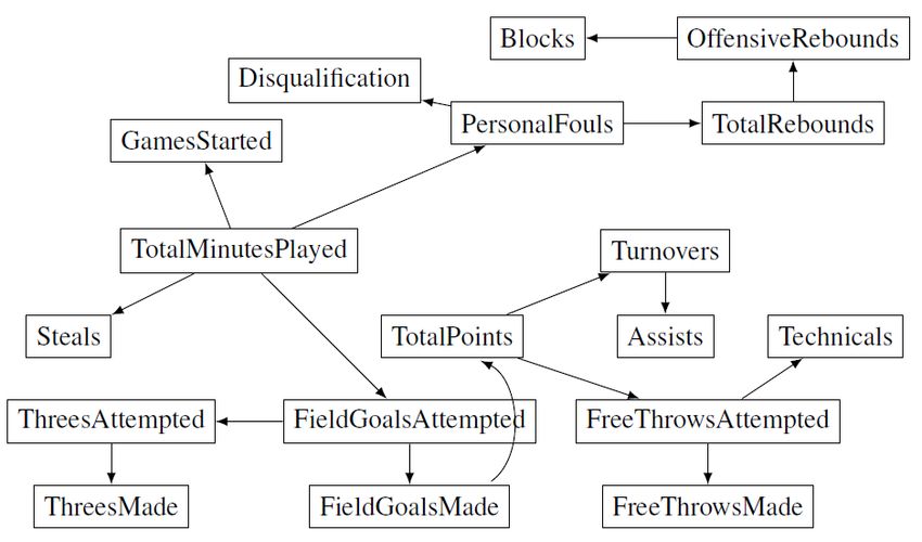
(a) DAG from MRS (b) DAG from ODS
(a) Hybrid: Precision (b) Hybrid: Recall
Figure 6: NBA players statistics DAG estimated by
Figure 5: Comparison of the MRS algorithms with the MRS (left) and DAG estimated by ODS (right).
different assumed node conditional distribution and
the GES algorithm in terms of recovering Hybrid DAG turnovers, blocks, personal fouls, disqualifications, tech-
models with p = 20. nicals fouls, games started and total points. We provide
the procedure of data preprocessing and the detailed
fixed node size p = 100, and (b) p ∈ {10, 20, ..., 200} summary of data in Supplementary.
with the fixed sample size n = 500. As we see in Fig. 4,
the time complexity of Step 1) is O(n2 p2 ), and that The MRS and ODS algorithms are applied where GES
of Step 2) of the MRS algorithm is O(np2 ). Hence we algorithm is used in Step 1). We assume that the
confirm the addition of estimation of ordering does not conditional distribution of each node given its par-
significantly add to the computational bottleneck. ents is hyper-Poisson because most of NBA statis-
tics we consider are the number of successes or at-
Deviations from True Distributions: When the tempts counted in the season. We emphasize that our
data are generated by a GHD DAG model where the method requires a known conditional distribution as-
conditional distribution of each node given its parents sumption to recover the true graph. However since we
is unknown, our algorithm is not guaranteed to esti- do not have prior node distribution information, we
mate the true graph and its ordering. Therefore, an set bj = Var(X
d j )/E(Xb j ) as we used in simulations that
important question is how well the MRS algorithm re- enables the MRS algorithm successfully recovers the
covers graphs when incorrect distributions are used. In directed edges.
this section, we heuristically investigate this question.
Fig. 6 shows the estimated directed graphs using
We use the same setting of the data generation for the MRS and ODS algorithms. There are 8 dis-
Hybrid GHD DAG models with the node size p = 20. tinct directed edges in the estimated DAG from the
We consider (i) the true (conditional) distributions, and MRS algorithm while the estimated DAG from the
assume all nodes (conditional) distributions are either ODS algorithm has opposite directions: TotalMinute-
(ii) Poisson; (iii) hyper-Poisson with b = 2; or (iv) hyper- sPlayed → PersonalFouls, Steals, and GamesStarted,
Poisson with b = Var(X)/
d E(X)
b that is an estimator ThreeAttempted → ThreeMade, TotalRebounds →
for the hyper-Poisson parameter b. We compare the OffensiveRebounds, OffensiveRebounds → Blocks,
MRS and GES algorithms by varying sample size n ∈ FreeThrowsAttempted → Technicals, and Personal-
{100, 200, ..., 1000} in Fig. 5. Fouls → Disqualification. The connections between
Fig. 5 shows that the MRS algorithms recover the true rebounds and blocks, and shooting attempted and tech-
graph better as sample size increases although there nicals do not makes sense in both directions, and hence
is no theoretical guarantees. It shows that the MRS they might be incorrectly estimated edges in Step 1).
algorithm enables to learn a part of ordering even if the However the remaining 6 directed edges are better
true (conditional) distributions are unknown as long explainable because the total minutes played would
as there are sufficient samples. be a reason for other statistics, and a large number of
shooting attempted would lead to the more shootings
4.2 Real Multivariate Count Data: made. It is consistent to our main point that MRS
2009/2010 NBA Player Statistics algorithm provides more legitimate directed edges than
the ODS algorithm by allowing a broader class of count
We demonstrate the advantages of our graphical mod- distributions.
els for count-valued data by learning 441 NBA player
statistics from season 2009/2010 (see R package Sport-
sAnalytics for detailed information). We consider 18 5 Acknowledgments
discrete variables: total minutes played, total number
of field goals made, field goals attempted, threes made, This work was supported by the National Research
threes attempted, free throws made, free throws at- Foundation of Korea(NRF) grant funded by the Korea
tempted, offensive rebounds, rebounds, assists, steals, government(MSIT) (NRF-2018R1C1B5085420).Gunwoong Park, Hyewon Park
References models. In Proceedings of the 26th annual interna-
tional conference on machine learning, pages 745–752.
Chickering, D. M. (2003). Optimal structure identifi-
ACM.
cation with greedy search. The Journal of Machine
Learning Research, 3:507–554. Park, G. and Raskutti, G. (2015). Learning large-scale
poisson dag models based on overdispersion scor-
Chickering, D. M., Geiger, D., Heckerman, D., et al. ing. In Advances in Neural Information Processing
(1994). Learning bayesian networks is np-hard. Tech- Systems, pages 631–639.
nical report, Citeseer.
Park, G. and Raskutti, G. (2017). Learning quadratic
Dacey, M. F. (1972). A family of discrete probability variance function (qvf) dag models via overdispersion
distributions defined by the generalized hypergeomet- scoring (ods). arXiv preprint arXiv:1704.08783.
ric series. Sankhyā: The Indian Journal of Statistics,
Series B, pages 243–250. Peters, J. and Bühlmann, P. (2014). Identifiability of
gaussian structural equation models with equal error
Friedman, N., Nachman, I., and Peér, D. (1999). Learn- variances. Biometrika, 101(1):219–228.
ing bayesian network structure from massive datasets:
Peters, J., Janzing, D., and Scholkopf, B. (2011).
the sparse candidate algorithm. In Proceedings of
Causal inference on discrete data using additive noise
the Fifteenth conference on Uncertainty in artificial
models. IEEE Transactions on Pattern Analysis and
intelligence, pages 206–215. Morgan Kaufmann Pub-
Machine Intelligence, 33(12):2436–2450.
lishers Inc.
Peters, J., Mooij, J., Janzing, D., and Schölkopf, B.
Frydenberg, M. (1990). The chain graph markov prop- (2012). Identifiability of causal graphs using func-
erty. Scandinavian Journal of Statistics, pages 333– tional models. arXiv preprint arXiv:1202.3757.
353.
Shimizu, S., Hoyer, P. O., Hyvärinen, A., and Ker-
Heckerman, D., Geiger, D., and Chickering, D. M. minen, A. (2006). A linear non-Gaussian acyclic
(1995). Learning Bayesian networks: The combi- model for causal discovery. The Journal of Machine
nation of knowledge and statistical data. Machine Learning Research, 7:2003–2030.
learning, 20(3):197–243.
Spirtes, P., Glymour, C. N., and Scheines, R. (2000).
Hoyer, P. O., Janzing, D., Mooij, J. M., Peters, J., Causation, prediction, and search. MIT press.
and Schölkopf, B. (2009). Nonlinear causal discovery
Tsamardinos, I. and Aliferis, C. F. (2003). Towards prin-
with additive noise models. In Advances in neural
cipled feature selection: Relevancy, filters and wrap-
information processing systems, pages 689–696.
pers. In Proceedings of the ninth international work-
Hyvärinen, A. and Smith, S. M. (2013). Pairwise likeli- shop on Artificial Intelligence and Statistics. Morgan
hood ratios for estimation of non-gaussian structural Kaufmann Publishers: Key West, FL, USA.
equation models. Journal of Machine Learning Re- Tsamardinos, I., Brown, L. E., and Aliferis, C. F. (2006).
search, 14(Jan):111–152. The max-min hill-climbing bayesian network struc-
Inouye, D. I., Yang, E., Allen, G. I., and Ravikumar, ture learning algorithm. Machine learning, 65(1):31–
P. (2017). A review of multivariate distributions for 78.
count data derived from the poisson distribution. Wi- Uhler, C., Raskutti, G., Bühlmann, P., and Yu, B.
ley Interdisciplinary Reviews: Computational Statis- (2013). Geometry of the faithfulness assumption in
tics, 9(3):e1398. causal inference. The Annals of Statistics, pages
Kemp, A. W. (1968). A wide class of discrete dis- 436–463.
tributions and the associated differential equations. Verma, T. and Pearl, J. (1992). An algorithm for decid-
Sankhyā: The Indian Journal of Statistics, Series A, ing if a set of observed independencies has a causal
pages 401–410. explanation. In Uncertainty in Artificial Intelligence,
Kemp, A. W. and Kemp, C. (1974). A family of dis- 1992, pages 323–330. Elsevier.
crete distributions defined via their factorial mo- Zhang, J. and Spirtes, P. (2016). The three faces of
ments. Communications in Statistics-Theory and faithfulness. Synthese, 193(4):1011–1027.
Methods, 3(12):1187–1196. Zhang, K. and Hyvärinen, A. (2009). On the iden-
Lauritzen, S. L. (1996). Graphical models. Oxford tifiability of the post-nonlinear causal model. In
University Press. Proceedings of the twenty-fifth conference on uncer-
tainty in artificial intelligence, pages 647–655. AUAI
Mooij, J., Janzing, D., Peters, J., and Schölkopf, B.
Press.
(2009). Regression by dependence minimization and
its application to causal inference in additive noiseYou can also read