Model Trees for Identifying Exceptional Players in the NHL Draft
←
→
Page content transcription
If your browser does not render page correctly, please read the page content below
Model Trees for Identifying Exceptional Players in
                                                           the NHL Draft
                                                                   Oliver Schulte1 , Yejia Liu2 , and Chao Li3
                                                    1,2,3
                                                            Department of Computing Science, Simon Fraser University
                                                                    {oschulte, yejial, chao_li_2}@sfu.ca

                                                                                  February 27, 2018
arXiv:1802.08765v1 [cs.LG] 23 Feb 2018

                                                                                        Abstract
                                                  Drafting strong players is crucial for a team’s success. We describe a new data-driven in-
                                              terpretable approach for assessing draft prospects in the National Hockey League. Successful
                                              previous approaches have 1) built a predictive model based on player features (e.g. Schuckers
                                              2017 [ESSC16], or 2) derived performance predictions from the observed performance of com-
                                              parable players in a cohort (Weissbock 2015 [W15]). This paper develops model tree learning,
                                              which incorporates strengths of both model-based and cohort-based approaches. A model tree
                                              partitions the feature space according to the values of discrete features, or learned thresholds
                                              for continuous features. Each leaf node in the tree defines a group of players, easily described
                                              to hockey experts, with its own group regression model. Compared to a single model, the
                                              model tree forms an ensemble that increases predictive power. Compared to cohort-based
                                              approaches, the groups of comparables are discovered from the data, without requiring a
                                              similarity metric. The performance predictions of the model tree are competitive with the
                                              state-of-the-art methods, which validates our model empirically. We show in case studies that
                                              the model tree player ranking can be used to highlight strong and weak points of players.

                                         1    Introduction
                                         Player ranking is one of the most studied subjects in sports analytics [AGSK13]. In this paper we
                                         consider predicting success in the National Hockey League(NHL) from junior league data, with the
                                         goal of supporting draft decisions. The publicly available junior league data aggregate a season’s
                                         performance into a single set of numbers for each player. Our method can be applied to any data
                                         of this type, for example also to basketball NBA draft data(www.basketball-reference.com/
                                         draft/). Since our goal is to support draft decisions by teams, we ensure that the results of our
                                         data analysis method can be easily explained to and interpreted by sports experts.
                                             Previous approaches for analyzing hockey draft data take a regression approach or a similarity-
                                         based approach. Regression approaches build a predictive model that takes as input a set of
                                         player features, such as demographics (age, height, weight) and junior league performance metrics
                                         (goals scored, plus-minus), and output a predicted success metric (e.g. number of games played
                                         in the professional league). The current state-of-the-art is a generalized additive model [ESSC16].
                                         Cohort-based approaches divide players into groups of comparables and predict future success
                                         based on a player’s cohort. For example, the PCS model [W15] clusters players according to age,
                                         height, and scoring rates. One advantage of the cohort model is that predictions can be explained
                                         by reference to similar known players, which many domain experts find intuitive. For this reason,
                                         several commercial sports analytics systems, such as Sony’s Hawk-Eye system, identify groups of
                                         comparables for each player. Our aim in this paper is to describe a new model for draft data that
                                         achieves the best of both approaches, regression-based and similarity-based.
                                             Our method uses a model tree [FHT00, Loh17]. Each node in the tree defines a new yes/no
                                         question, until a leaf is reached. Depending on the answers to the questions, each player is assigned
                                         a group corresponding to a leaf. The tree builds a different regression model for each leaf node.
                                         Figure 1 shows an example model tree. A model tree offers several advantages.

                                                                                             1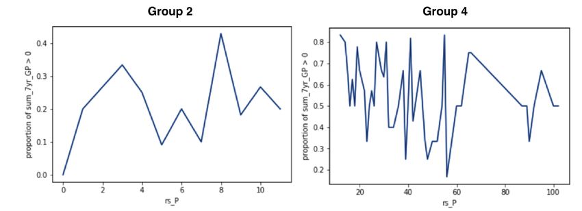
Figure 1: Logistic Regression Model Trees for the 2004, 2005, 2006 cohort in NHL. The tree was
built using the LogitBoost algorithm implemented in the LMT package of the Weka Program
[FHW16, HFH+ 09].

   • Compared to a single regression model, the tree defines an ensemble of regression models,
     based on non-linear thresholds. This increases the expressive power and predictive accuracy
     of the model. The tree can represent complex interactions between player features and
     player groups. For example, if the data indicate that players from different junior leagues
     are sufficiently different to warrant building distinct models, the tree can introduce a split to
     distinguish different leagues.

   • Compare to a similarity-based model, tree construction learns groups of players from the
     data, without requiring the analyst to specify a similarity metric. Because tree learning
     selects splits that increase predictive accuracy, the learned distinctions between the groups
     are guaranteed to be predictively relevant to future NHL success. Also, the tree creates a
     model, not a single prediction, for each group, which allows it to differentiate players from
     the same group.

    A natural approach would be to build a linear regression tree to predict NHL success, which
could be measured by the number of games a draft pick plays in the NHL. However, only about
half the draft picks ever play a game in the NHL [TMM11]. As observed by [ESSC16], this creates
a zero-inflation problem that limits the predictive power of linear regression. We propose a novel
solution to the zero-inflation problem, which applies logistic regression to predict whether a player
will play at least one game in the NHL. We learn a logistic regression model tree, and rank players
by the probability that the logistic regression model tree assigns to them playing at least one
game. Intuitively, if we can be confident that a player will play at least one NHL game, we can
also expect the player to play many NHL games. Empirically, we found that on the NHL draft
data, the logistic regression tree produces a much more accurate player ranking than the linear
regression tree.
    Following [ESSC16], we evaluate the logistic regression ranking by comparing it to ranking
players by their future success, measured as the number of NHL games they play after 7 years.
The correlation of the logistic regression ranking with future success is competitive with that

                                                  2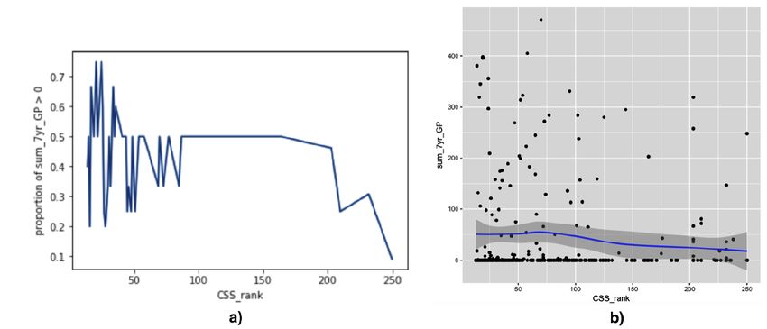
achieved by the generalized additive model of [ESSC16]. We show in case studies that the logistic
model tree adds information to the NHL’s Central Scouting Service Rank (CSS). For example,
Stanley Cup winner Kyle Cumiskey was not ranked by the CSS in his draft year, but was ranked
as the third draft prospect in his group by the model tree, just behind Brad Marchand and Mathieu
Carle. Our case studies also show that the feature weights learned from the data can be used to
explain the ranking in terms of which player features contribute the most to an above-average
ranking. In this way the model tree can be used to highlight exceptional features of a player for
scouts and teams to take into account in their evaluation.
    Paper Outline. After we review related work, we show and discuss the model tree learned from
the 2004-2006 draft data. The rank correlations are reported to evaluate predictive accuracy. We
discuss in detail how the ensemble of group models represents a rich set of interactions between
player features, player categories, and NHL success. Case studies give examples of strong players
in different groups and show how the model can used to highlight exceptional player features.

2    Related Work
Different approaches to player ranking are appropriate for different data types. For example, with
dynamic play-by-play data, Markov models have been used to rank players [CDBG16, TVJM13,
SZS17, KMR14]. For data that record the presence of players when a goal is scored, regression
models have also been applied to extend the classic plus-minus metric [Mac11, GJT13]. In this
paper, we utilize player statistics that aggregate a season’s performance into a single set of numbers.
While this data is much less informative than play-by-play data, it is easier to obtain, interpret,
and process.
    Regression Approaches. To our knowledge, this is the first application of model trees to hockey
draft prediction, and the first model for predicting whether a draftee plays any games at all. The
closest predecessor to our work is due to Schuckers [ESSC16], who uses a single generalized additive
model to predict future NHL game counts from junior league data.
    Similarity-Based Approaches assume a similarity metric and group similar players to predict
performance. A sophisticated example from baseball is the nearest neighbour analysis in the
PECOTA system [Sil04]. For ice hockey, the Prospect Cohort Success (PCS) model [W15], cohorts
of draftees are defined based on age, height, and scoring rates. Model tree learning provides an
automatic method for identifying cohorts with predictive validity. We refer to cohorts as groups
to avoid confusion with the PCS concept. Because tree learning is computationally efficient, our
model tree is able to take into account a larger set of features than age, height, and scoring rates.
Also, it provides a separate predictive model for each group that assigns group-specific weights to
different features. In contrast, PCS makes the same prediction for all players in the same cohort.
So far, PCS has been applied to predict whether a player will score more than 200 games career
total. Tree learning can easily be modified to make predictions for any game count threshold.

3    Dataset
Our data was obtained from public-domain on-line sources, including nhl.com, eliteprospects.
com, and draftanalyst.com. We are also indebted to David Wilson for sharing his NHL perfor-
mance dataset [Wil16]. The full dataset is posted on the Github(https://github.com/liuyejia/
Model_Trees_Full_Dataset). We consider players drafted into the NHL between 1998 to 2008
(excluding goalies). Following [ESSC16], we took as our dependent variable the total number of
games gi played by a player i after 7 years under an NHL contract. The first seven seasons are
chosen because NHL teams have at least seven-year rights to players after they are drafted [SC13].
Our dataset includes also the total time on ice after 7 years. The results for time on ice were very
similar to number of games, so we discuss only the results for number of games. The independent
variables include demographic factors (e.g. age), performance metrics for the year in which a player
was drafted (e.g., goals scored), and the rank assigned to a player by the NHL Central Scouting
Service (CSS). If a player was not ranked by the CSS, we assigned (1+ the maximum rank for his
draft year) to his CSS rank value. Another preprocessing step was to pool all European countries
into a single category. If a player played for more than one team in his draft year (e.g., a league
team and a national team), we added up this counts from different teams. Table 1 lists all data
columns and their meaning. Figure 1 shows an excerpt from the dataset.

                                                  3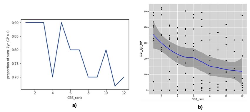
Variable Name                 Description
 id                            nhl.com id for NHL players, otherwise Eliteprospects.com id
 DraftAge                      Age in Draft Year
 Country                       Nationality. Canada -> ’CAN’, USA -> ’USA’, countries in Eu-
                               rope -> ’EURO’
 Position                      Position in Draft Year. Left Wing -> ’L’, Right Wing -> ’R’,
                               Center -> ’C’, Defencemen -> ’D’
 Overall                       Overall pick in NHL Entry Draft
 CSS_rank                      Central scouting service ranking in Draft Year
 rs_GP                         Games played in regular seasons in Draft Year
 rs_G                          Goals in regular seasons in Draft Year
 rs_A                          Assists in regular seasons in Draft Year
 rs_P                          Points in regular seasons in Draft Year
 rs_PIM                        Penalty Minutes in regular seasons in Draft Year
 rs_PlusMinus                  Goal Differential in regular seasons in Draft Year
 po_GP                         Games played in playoffs in Draft Year
 po_G                          Goals in playoffs in Draft Year
 po_A                          Assists in playoffs in Draft Year
 po_P                          Points in playoffs in Draft Year
 po_PIM                        Penalty Minutes in playoffs in Draft Year
 po_PlusMinus                  Goal differential in playoffs in Draft Year
 sum_7yr_GP                    Total NHL games played in player’s first 7 years of NHL career
 sum_7yr_TOI                   Total NHL Time on Ice in player’s first 7 years of NHL career
 GP_7yr_greater_than_0         Played a game or not in player’s first 7 years of NHL career

            Table 1: Player Attributes listed in dataset (excluding weight and height).

Figure 2: Sample Player Data for their draft year. rs = regular season. We use the same statistics
for the playoffs (not shown).

4    Model Tree Construction
Model trees are a flexible formalism that can be built for any regression model. An obvious
candidate for a regression model would be linear regression; alternatives include a generalized
additive model [ESSC16], and a Poisson regression model specially built for predicting counts
[Ryd04]. We introduce a different approach: a logistic regression model to predict whether a
player will play any games at all in the NHL (gi > 0). The motivation is that many players in the
draft never play any NHL games at all (up to 50% depending on the draft year) [TMM11]. This
poses an extreme zero-inflation problem for any regression model that aims to predict directly the
number of games played. In contrast, for the classification problem of predicting whether a player
will play any NHL games, zero-inflation means that the data set is balanced between the classes.
This classification problem is interesting in itself; for instance, a player agent would be keen to
know what chances their client has to participate in the NHL. The logistic regression probabilities
pi = P (gi > 0) can be used not only to predict whether a player will play any NHL games, but
also to rank players such that the ranking correlates well with the actual number of games played.
Our method is therefore summarized as follows.

                                                4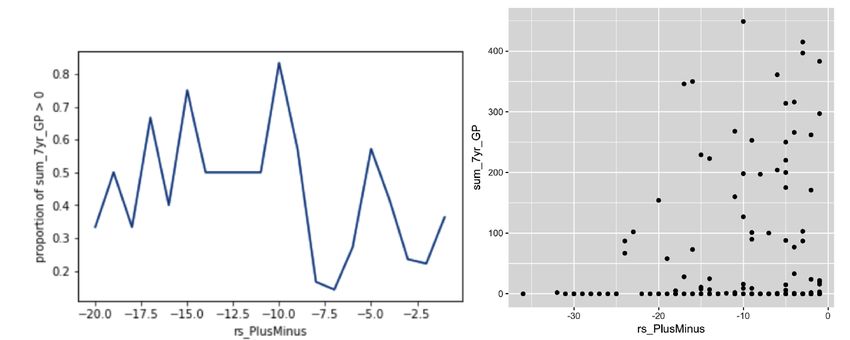
1. Build a tree whose leaves contain a logistic regression model.
    2. The tree assigns each player i to a unique leaf node li , with a logistic regression model m(li ).
    3. Use m(li ) to compute a probability pi = P (gi > 0).

    Figure 1 shows the logistic regression model tree learned for our second cohort by the LogiBoost
algorithm. It places CSS rank at the root as the most important attribute. Players ranked better
than 12 form an elite group, of whom almost 82% play at least one NHL games. For players at
rank 12 or below, the tree considers next their regular season points total. Players with rank and
total points below 12 form an unpromising group: only 16% of them play an NHL game. Players
with rank below 12 but whose points total is 12 or higher, are divided by the tree into three groups
according to whether their regular season plus-minus score is positive, negative, or 0. (A three-way
split is represented by two binary splits). If the plus-minus score is negative, the prospects of
playing an NHL game are fairly low at about 37%. For a neutral plus-minus score, this increases
to 61%. For players with a positive plus-minus score, the tree uses the number of playoff assists
as the next most important attribute. Players with a positive plus-minus score and more than 10
playoff assists form a small but strong group that is 92% likely to play at least one NHL game.

5     Results: Predictive Modelling
Following [ESSC16], we evaluated the predictive accuracy of the LMT model using the Spearman
Rank Correlation(SRC) between two player rankings: i) the performance ranking based on the
actual number of NHL games that a player played, and ii) the ranking of players based on the
probability pi of playing at least one game(Tree Model SRC). We also compared it with iii) the
ranking of players based on the order in which they were drafted (Draft Order SRC). The draft
order can be viewed as the ranking that reflects the judgment of NHL teams. We provide the
formula for the Spearman correlation in the Appendix. Table 2 shows the Spearman correlation
for different rankings.

         Training Data       Out of Sample     Draft Order               LMT              LMT
        NHL Draft Years       Draft Years         SRC          Classification Accuracy    SRC
        1998, 1999, 2000         2001             0.43                  82.27%             0.83
        1998, 1999, 2000         2002             0.30                  85.79%             0.85
        2004, 2005, 2006         2007             0.46                  81.23%             0.84
        2004, 2005, 2006         2008             0.51                  63.56%             0.71

Table 2: Predictive Performance (our Logitic Model Trees, over all draft ranking) using Spearman
Rank Correlation. Bold indicates the best values.

    Other Approaches. We also tried designs based on a linear regression model tree, using the
M5P algorithm implemented in the Weka program. The result is a decision stump that splits on
CSS rank only, which had substantially worse predictive performance(i.e., Spearman correlation
of only 0.4 for the 2004 − 2006 cohort). For the generalized additive model (gam), the reported
correlations were 2001 : 0.53, 2002 : 0.54, 2007 : 0.69, 2008 : 0.71 [ESSC16]. Our correlation is not
directly comparable to the gam model because of differences in data preparation: the gam model
was applied only to drafted players who played at least one NHL game, and the CSS rank was
replaced by the Cescin conversion factors: for North American players, multiply CSS rank by 1.35,
and for European players, by 6.27 [Fyf11]. The Cescin conversion factors represent an interaction
between the player’s country and the player’s CSS rank. A model tree offers another approach
to representing such interactions: by splitting on the player location node, the tree can build a
different model for each location. Whether the data warrant building different models for different
locations is a data-driven decision made by the tree building algorithm. The same point applies to
other sources of variability, for example the draft year or the junior league. Including the junior
league as a feature has the potential to lead to insights about the differences between leagues,
but would make the tree more difficult to interpret; we leave this topic for future work. In the
next section we examine the interaction effects captured by the model tree in the different models
learned in each leaf node.

                                                   5
6 Results: Learned Groups and Logistic Regression Models
We examine the learned group regression models, first in terms of the dependent success variable,
then in terms of the player features.
6.1 Groups and the Dependent Variable
Figure 3 shows boxplots for the distribution of our dependent variable gi . The strongest groups
are, in order, 1, 6, and 4. The other groups show weaker performance on the whole, although in
each group some players reach high numbers of games. Most players in Group 2&3&4&5 have
GP equals to zero while Group 1&6 represent the strongest cohort in our prediction, where over
80% players played at least 1 game in NHL. The tree identifies that among the players who do
not have a very high CSS rank (worse than 12), the combination of regular season P oints >= 12,
P lusM inus > 0, and play − of f Assists > 10 is a strong indicator of playing a substantive number
of NHL games (median gi = 128).
Figure 3: Boxplots for the dependent variable gi , the total number of NHL games played after 7
years under an NHL contract. Each boxplot shows the distribution for one of the groups learned
by the logistic regression model tree. The group size is denoted n.
6.2 Groups and the Independent Variables
Figure 5.2 shows the average statistics by group and for all players. The CSS rank for Group 1
is by far the highest. The data validate the high ranking in that 82% players in this group went
on to play an NHL game. Group 6 in fact attains an even higher proportion of 92%. The average
statistics of this group are even more impressive than those of group 1 (e.g., 67 regular season
points in group 6 vs. 47 for group 1). But the average CSS rank is the lowest of all groups. So
this group may represent a small group of players (n = 13) overlooked by the scouts but identified
by the tree. Other than Group 6, the group with the lowest CSS rank on average is Group 2. The
data validate the low ranking in that only 16% of players in this group went on to play an NHL
game. The group averages are also low (e.g., 6 regular season points is much lower than other
groups).
6Figure 4: Statistics for the average players in each group and all players.
7 Group Models and Variable Interactions
Figure 5 illustrates logistic regression weights by group. A positive weight implies that an increase
in the covariate value predicts a large increase in the probability of playing more than one game,
compared to the probability of playing zero games. Conversely, a negative weight implies that an
increase in the covariate value decreases the predicted probability of playing more than one game.
Bold numbers show the groups for which an attribute is most relevant. The table exhibits many
interesting interactions among the independent variables; we discuss only a few. Notice that if
the tree splits on an attribute, the attribute is assigned a high-magnitude regression weight by
the logistic regression model for the relevant group. Therefore our discussion focuses on the tree
attributes.
Figure 5: Group 200(4 + 5 + 6 + 7 + 8) Weights Illustration. E = Europe, C = Canada, U
= USA, rs = Regular Season, po = Playoff. Largest-magnitude weights are in bold. Underlined
weights are discussed in the text.
At the tree root, CSS rank receives a large negative weight of −17.9 for identifying the most
successful players in Group 1, where all CSS ranks are better than 12. Figure 6a shows that the
proportion of above-zero to zero-game players decreases quickly in Group 1 with worse CSS rank.
However, the decrease is not monotonic. Figure 6b is a scatterplot of the original data for Group
1. We see a strong linear correlation (p = −0.39), and also a large variance within each rank.
The proportion aggregates the individual data points at a given rank, thereby eliminating the
variance. This makes the proportion a smoother dependent variable than the individual counts for
a regression model.
Group 5 has the smallest logistic regression coefficient of −0.65. Group 5 consists of players
7Figure 6: Proportion and scatter plots for CSS_rank vs. sum_7yr_GP in Group 1.
whose CSS ranks are worse than 12, regular season points above 12, and plus-minus above 1.
Figure 7a plots CSS rank vs. above-zero proportion for Group 5. As the proportion plot shows,
the low weight is due to the fact that the proportion trends downward only at ranks worse than
200. The scatterplot in Figure 7b shows a similarly weak linear correlation of −0.12.
Figure 7: Proportion and scatter plots for CSS_rank vs.sum_7yr_GP in Group 5.
Regular season points are the most important predictor for Group 2, which comprises players
with CSS rank worse than 12, and regular season points below 12. In the proportion plot Figure
8, we see a strong relationship between points and the chance of playing more than 0 games
(logistic regression weight 14.2). In contrast in Group 4 (overall weight −1.4), there is essentially
no relationship up to 65 points; for players with points between 65 and 85 in fact the chance of
playing more than zero games slightly decreases with increasing points.
In Group 3, players are ranked at level 12 or worse, have collected at least 12 regular season
points, and show a negative plus-minus score. The most important feature for Group 3 is the
regular season plus-minus score (logistic regression weight 13.16), which is negative for all players
in this group. In this group, the chances of playing an NHL game increase with plus-minus, but
not monotonically, as Figure 9 shows.
For regular season goals, Group 5 assigns a high logistic regression weight of 3.59. However,
Group 2 assigns a surprisingly negative weight of −2.17. Group 5 comprises players at CSS rank
worse than 12, regular season points 12 or higher, and positive plus-minus greater than 1. About
8Figure 8: Proportion_of_Sum_7yr_GP_greater_than_0 vs. rs_P in Group 2&4.
Figure 9: Proportion and scatter plots for rs_PlusMinus vs.sum_7yr_GP in group 3.
64.8% in this group are offensive players (see Figure 10). The positive weight therefore indicates
that successful forwards score many goals, as we would expect.
Group 2 contains mainly defensemen (61.6%; see Figure 10). The typical strong defenseman
scores 0 or 1 goals in this group. Players with more goals tend to be forwards, who are weaker in
this group. In sum, the tree assigns weights to goals that are appropriate for different positions,
using statistics that correlate with position (e.g., plus-minus), rather than the position directly.
8 Identifying Exceptional Players
Teams make drafting decisions not based on player statistics alone, but drawing on all relevant
source of information, and with extensive input from scouts and other experts. As Cameron
Lawrence from the Florida Panthers put it, ‘the numbers are often just the start of the discussion’[JL17].
In this section we discuss how the model tree can be applied to support the discussion of individual
players by highlighting their special strengths. The idea is that the learned weights can be used
to identify which features of a highly-ranked player differentiate him the most from others in his
group.
Explaining the Rankings: identify weak points and strong points
Our method is as follows. For each group, we find the average feature vector of the players in the
group, which we denote by xg1 , xg2 , ..., xgm (see Figure 4). We denote the features of player i as
xi1 , xi2 , ..., xim . Then given a weight vector (w1 , wm ) for the logistic regression model of group g,
9Figure 10: Distribution of Defenseman vs. Forwards in Group 5&2. The size is denoted as n.
the log-odds difference between player i and a random player in the group is given by
Pm
j=1 wj (xij − xgi )
We can interpret this sum as a measure of how high the model ranks player i compared to
other players in his group. This suggests defining as the player’s strongest features the xij that
maximize wj (xij − xgi ), and as his weakest features those that minimize wj (xij − xgi ). This
approach highlights features that are i) relevant to predicting future success, as measured by the
magnitude of wj , and ii) different from the average value in the player’s group of comparables, as
measured by the magnitude of xij − xgi .
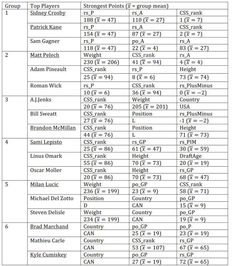
Case Studies
Figure 11 shows, for each group, the three strongest points for the most highly ranked players
in the group. We see that the ranking for individual players is based on different features, even
within the same group. The table also illustrates how the model allows us to identify a group of
comparables for a given player. We discuss a few selected players and their strong points. The
most interesting cases are often those where are ranking differs from the scouts’ CSS rank. We
therefore discuss the groups with lower rank first.
Among the players who were not ranked by CSS at all, our model ranks Kyle Cumiskey at the
top. Cumiskey was drafted in place 222, played 132 NHL games in his first 7 years, represented
Canada in the World Championship, and won a Stanley Cup in 2015 with the Blackhawks. His
strongest points were being Canadian, and the number of games played (e.g., 27 playoff games vs.
19 group average).
In the lowest CSS-rank group 6 (average 107), our top-ranked player Brad Marchand received
CSS rank 80, even below his Boston Bruin teammate Lucic’s. Given his Stanley Cup win and
success representing Canada, arguably our model was correct to identify him as a strong NHL
prospect. The model highlights his superior play-off performance, both in terms of games played
and points scored. Group 2 (CSS average 94) is a much weaker group. Matt Pelech is ranked at
the top by our model because of his unusual weight, which in this group is unusually predictive of
NHL participation. In group 4 (CSS average 86), Sami Lepisto was top-ranked, in part because
he did not suffer many penalties although he played a high number of games. In group 3 (CSS
average 76), Brandon McMillan is ranked relatively high by our model compared to the CSS. This
is because in this group, left-wingers and shorter players are more likely to play in the NHL. In
our ranking, Milan Lucic tops Group 5 (CSS average 71). At 58, his CSS rank is above average
10in this group, but much below the highest CSS rank player (Legein at 13). The main factors for
the tree model are his high weight and number of play-off games played. Given his future success
(Stanley Cup, NHL Young Stars Game), arguably our model correctly identified him as a star in
an otherwise weaker group. The top players in Group 1 like Sidney Crosby and Patrick Kane are
obvious stars, who have outstanding statistics even relative to other players in this strong group.
Figure 11: Strongest Statistics for the top players in each group. Underlined players are discussed
in the text.
9 Conclusion and Future Work
We have proposed building a regression model tree for ranking draftees in the NHL, or other
sports, based on a list of player features and performance statistics. The model tree groups players
according to the values of discrete features, or learned thresholds for continuous performance
statistics. Each leaf node defines a group of players that is assigned its own regression model.
Tree models combine the strength of both regression and cohort-based approaches, where player
performance is predicted with reference to comparable players. An obvious approach is to use a
linear regression tree for predicting our dependent variable, the number of NHL games played by a
player within 7 NHL years. However, we found that a linear regression tree performs poorly due to
the zero-inflation problem (many draft picks never play any NHL game). Instead, we introduced
the idea of using a logistic regression tree to predict whether a player plays any NHL game within
7 years. Players are ranked according to the model tree probability that they play at least 1 game.
Key findings include the following. 1) The model tree ranking correlates well with the actual
success ranking according to the actual number of games played: better than draft order and com-
petitive with the state-of-the-art generalized additive model [ESSC16]. 2) The model predictions
complement the Central Scouting Service (CSS) rank. For example, the tree identifies a group
whose average CSS rank is only 107, but whose median number of games played after 7 years is
128, including several Stanley Cup winners. 3) The model tree can highlight the exceptionally
strong and weak points of draftees that make them stand out compared to the other players in
their group.
Tree models are flexible and can be applied to other prediction problems to discover groups of
comparable players as well as predictive models. For example, we can predict future NHL success
11from past NHL success, similar to Wilson [Wil16] who used machine learning models to predict
whether a player will play more than 160 games in the NHL after 7 years. Another direction is to
apply the model to other sports, for example drafting for the National Basketball Association.
References
[AGSK13] J. Albert, M. E. Glickman, T. B. Swartz, and R. H. Koning. Handbook of Statistical
Methods and Analyses in Sports. CRC Press, 2013.
[CDBG16] D. Cervone, A. D’Amour, L. Bornn, and K. Goldsberry. Pointwise: Prediting points
and valuing decisons in real time with nba optical tracking data. In MIT sloan Sports
Analytics Conference, 2016.
[Che96] K. J. Cherkauer. Human expert-level performance on a scientific image analysis task
by a system using combined artificial neural networks. In In Chan, P. (Ed.), Working
Notes of AAAI Workshop on Integrating Multiple Learned Model, pages 15–21, 1996.
[ESSC16] Michael E.Schuckers and LLC Statistical Sports Consulting. Draft by numbers: Using
data and analytics to improve national hockey league(NHL) player selection. In MIT
sloan Sports Analytics Conference, 2016.
[FHP57] E. C. Fieller, H. O. Hartley, and E. S. Pearson. Tests for rank correlation coefficients.
i. Biometrika, 44:470–481, 1957.
[FHT00] J. Friedman, T. Hastie, and R. Tibshirani. Additive logistic regression: A statistical
view of boosting. The Annals of Statistics, 28(2):337–407, 2000.
[FHW16] E. Frank, M. Hall, and I. Witten. The Weka Workbench. Online Appendix for Data
Mining: Practical Machine Learning Tools and Techniques. Fourth edition, 2016.
[FS] Y. Freund and R. E. Schapire. Experiments with a new boosting algorithm. In In Proc.
13th International Conference on Machine Learning, pages 148–146.
[Fyf11] Iain Fyffe. Evaluating central scouting. Technical report, 2011.
[GJT13] R. Gramacy, S. Jesen, and M. Taddy. Estimating player contribution in hockey with
regularized logistic regression. J Quant Anal Sports, pages 97–111, 2013.
[HFH+ 09] M. Hall, E. Frank, G. Homes, B. Pfahringer, P. Reutemann, and I. Witten. The weka
data mining software: An update. sigkdd explorations. 11:10–18, 2009.
[JL17] Eric Joyce and Cameron Lawrence. Blending old and new: How the florida panthers
try to predict future performance at the nhl entry draft, 2017.
[KMR14] E.H. Kaplan, K. Masri, and J.T. Ryan. A markov game model for hockey: Manpower
differential and win probability added. INFOR: Information Systems and Operational
Research, 52(2):39–50, 2014.
[Loh17] Wei-Yin Loh. GUIDE User Manual. University of Wisconsin-Madison, 2017.
[Mac11] B. Macdonald. An improved adjusted plus-minus statistic for nhl players. In MIT sloan
Sports Analytics Conference, 2011.
[Ryd04] Alan Ryder. Poisson toolbox, a review of the application of the poisson probability
distribution in hockey. Technical report, Hockey Analytics, 2004.
[SC13] Michael Schuckers and James Curro. Total hockey rating (thor): A comprehensive
statistical rating of national hockey league forwards and defensemen based upon all
on-ice events. In MIT sloan Sports Analytics Conference, 2013.
[Sil04] Nate Silver. PECOTA 2004: A Look Back and a Look Ahead, pages 5–10. New York:
Workman Publishers, 2004.
12[SZS17] O. Schulte, Z. Zhao, and SPORTLOGiQ. Apples-to-apples: Clustering and ranking nhl
players using location information and scoring impact. In MIT sloan Sports Analytics
Conference, 2017.
[TMM11] P. Tingling, K. Masri, and M. Martell. Does order matter? an empirical analysis
of nhl draft decisions. Sport, Business and Management: an International Journal,
(2):155–171, 2011.
[TVJM13] A. Thomas, S. Ventural, S. Jensen, and S. Ma. Competing process hazard function
model for player ratings in ice hockey. The Annals of Applied Science, 7(2):1497–1524,
2013.
[W15] Josh W. Draft analytics: Unveiling the prospect cohort success model. Technical
report, 2015.
[Wil16] David Wilson. Mining nhl draft data and a new value pick chart. Master’s thesis,
University of Ottawa, 2016.
Appendices
Spearman Rank Correlation
Spearman’s correlation measures the relevance and direction of monotonic association between two
variables [FHP57].PThe standard formula for calculating is based on the squared rank differences:
6 d2i
(1) p = 1 − n(n2 −1) , formula for no tied ranks. n = number of ranks, di = difference in paired
ranks. This is the
P formula we applied in Table 3.
(x −x)(y −y)
(2) p = √P i i 2 P i 2
, where xi = rank of player i according to ranking x, ditto for yi .
i (xi −x) i (yi −y )
Players who have played zero NHL games are tied when ranked by the number of NHL games;
this is the only case of ties. Table 3 repeats the calculation of Table 2 using the Pearson correlation
among ranks (2) rather than the squared rank differences (1). With this measure also, the model
ranking correlates more highly with actual number of games played than the team draft order.
Training Data Out of Sample Draft Order Tree Model
NHL Draft Years Draft Years Pearson Correlation Pearson Correlation
1998, 1999, 2000 2001 0.43 0.69
1998, 1999, 2000 2002 0.45 0.72
2004, 2005, 2006 2007 0.48 0.60
2004, 2005, 2006 2008 0.51 0.58
Table 3: Pearson Correlation of NHL ranks.
LogitBoost Algorithm
Ensemble methods provide a combination of classifiers to obtain a better predictive result than
any of the standalone constituents [Ryd04, FS, Che96]. While a model tree constructs a set of
different classifiers, it also partitions the space of players, so the prediction for each player is
based on exactly one model only, rather than a weighted majority vote. The LogitBoost algorithm
[FHT00] combines a model tree with weighted votes by building a separate model for each tree
node (including non-leaf nodes). The prediction for a specific player is then the weighted vote
of all models along the branch assigned to the player. This offers some of the advantages of a
hierarchical shrinkage model in smoothing parameter values so that predictions from players from
similar groups tend to use similar weights. In this paper, we used the tree structure learned from
LogitBoost, with simple maximum likelihood estimates for the weights to make the weight for a leaf
more interpretable by fitting the data in the leaf’s group more closely. The GUIDE system [Loh17]
is a well-developed software package that supports building ensembles of model trees. While such
13an ensemble tends to have even higher predictive accuracy, we have in this paper built only a single
model tree to maintain interpretability.
14You can also read