Location-based species recommendation using co-occurrences and environment-GeoLifeCLEF 2018 challenge - CEUR Workshop Proceedings
←
→
Page content transcription
If your browser does not render page correctly, please read the page content below
Location-based species recommendation using
 co-occurrences and environment- GeoLifeCLEF
                 2018 challenge

    Benjamin Deneu1 , Maximilien Servajean2 , Christophe Botella3 , and Alexis
                                     Joly1
                         1
                           Inria, LIRMM, Montpellier, France
                   alexis.joly@inria.fr benjamin.deneu@inria.fr
                      2
                        AMIS, Université Paul Valéry Montpellier
                 LIRMM UMR 5506, CNRS, University of Montpellier
                          maximilien.servajean@lirmm.fr
                 3
                    INRA, Inria, AMAP, LIRMM, Montpellier, France
                            christophe.botella@inria.fr

        Abstract. This paper presents several approaches for plant predictions
        given their location in the context of the GeoLifeCLEF 2018 challenge.
        We have developed three kinds of prediction models, one convolutional
        neural network on environmental data (CNN), one neural network on
        co-occurrences data and two other models only based on the spatial
        occurrences of species (a closest-location classifier and a random forest
        fitted on the spatial coordinates). We also evaluated the combination of
        these models through two different late fusion methods (one based on
        predictive probabilities and the other one based on predictive ranks).
        Results show the effectiveness of the CNN which obtained the best pre-
        diction score of the whole GeoLifeCLEF challenge. The fusion of this
        model with the spatial ones only provides slight improvements suggest-
        ing that the CNN already captured most of the spatial information in
        addition to the environmental preferences of the plants.

1     Introduction
Automatically predicting the list of species that are the most likely to be ob-
served at a given location is useful for many scenarios in biodiversity informatics.
First of all, it could improve species identification processes and tools by reduc-
ing the list of candidate species that are observable at a given location (be they
automated, semi-automated or based on classical field guides or flora). More
generally, it could facilitate biodiversity inventories through the development of
location-based recommendation services (typically on mobile phones) as well as
the involvement of non-expert nature observers. Last but not least, it might
serve educational purposes thanks to biodiversity discovery applications provid-
ing innovative features such as contextualized educational pathways.
This challenge is highly related to the problem known as Species Distribution
Modeling (SDM) in ecology. SDM have become increasingly important in the last
few decades for the study of biodiversity, macro ecology, community ecology and the ecology of conservation. An accurate knowledge of the spatial distribution of species is actually of crucial importance for many concrete scenarios including landscape management, preservation of rare and/or endangered species, surveil- lance of alien invasive species, measurement of human impact or climate change on species, etc. Concretely, the goal of SDM is to infer the spatial distribution of a given species, and they are often based on a set of geo-localized occurrences of that species (collected by naturalists, field ecologists, nature observers, citizen sciences project, etc.). However, it is usually not reliable to learn that distribu- tion directly from the spatial positions of the input occurrences. The two major problems are the limited number of occurrences and the bias of the sampling effort compared to the real underlying distribution. In a real-world dataset, the raw spatial distribution of the occurrences is actually highly influenced by the accessibility of the sites, the preferences and habits of the observers. Another difficulty is that an occurrence means a punctual presence of the species, while no occurrences doesn’t mean the species is absent, which makes us very uncer- tain about regions without observed specimens. For all these reasons, SDM is usually achieved through environmental niche modeling approaches, i.e. by predicting the distribution in the geographic space on the basis of a representation in the environmental space. This environmental space is in most cases represented by climate data (such as temperature, and precipitation), but also by other variables such as soil type, land cover, distance to water, etc. Then, the objective is to learn a function that takes the envi- ronmental feature vector of a given location as input and outputs an estimate of the abundance of the species. The main underlying hypothesis is that the abundance function is related to the fundamental ecological niche of the species. That means that in theory, a given species is likely to live in a single privileged ecological niche, characterized by an unimodal distribution in the environmental space. However, in reality, the abundance function is expected to be more com- plex. Many phenomena can actually affect the distribution of the species relative to its so called abiotic preferences. For instance, environment perturbations, or geographical constraints, or interactions with other living organisms (including humans) might have encourage specimens of that species to live in a different environment. As a consequence, the realized ecological niche of a species can be much more diverse and complex than its hypothetical fundamental niche. Very recently, SDM based on deep neural networks have started to appear [2]. These first experiments showed that they can have a good predictive power, po- tentially better than the models used conventionally in ecology. Actually, deep neural networks are able to learn complex nonlinear transformations in a wide variety of domains. In addition, they make it possible to learn an area of envi- ronmental representation common to a large number of species, which stabilizes predictions from one species to another and improves them globally. Finally, spatial patterns in environmental variables often contain useful information for species distribution but are generally not considered in conventional models. Conversely, convolutional neural networks effectively use this information and
improve prediction performance.
In this paper, we report an evaluation study of three main kinds of SDM in the
context of the GeoLifeCLEF challenge [1, 4]:
 1. A convolutional neural network aimed at learning the ecological preferences
    of species thanks to environmental image patches provided as inputs (tem-
    perature, soil type, etc.).
 2. A purely spatial model based on a random forest fitted on the spatial coor-
    dinates of the occurrences of each species.
 3. A species co-occurrence model aiming at predicting the likelihood of presence
    of a given species thanks to the knowledge of the presence of other species.
   Section 2 gives an overview of the data and evaluation methodology of the
GeoLifeCLEF challenge. Section 3 provides the detailed description of the evalu-
ated models. Section 4 presents the results of the experiments and their analysis.

2   Data and evaluation methodology
A detailed description of the protocol used to build the GeoLifeCLEF 2018
dataset is provided in [1]. In a nutshell, the dataset was built from occurrence
data of the Global Biodiversity Information Facility (GBIF), the world’s largest
open data infrastructure in this domain, funded by governments. It is com-
posed of 291,392 occurrences of N = 3, 336 plant species observed on the French
territory between 1835 and 2017. Each occurrence is characterized by 33 local
environmental images of 64x64 pixels. These environmental images are windows
cropped from wider environmental rasters and centered on the occurrence spatial
location. They were constructed from various open datasets including Chelsea
Climate, ESDB soil pedology data, Corine Land Cover 2012 soil occupation data,
CGIAR-CSI evapotranspiration data, USGS Elevation data (Data available from
the U.S. Geological Survey.) and BD Carthage hydrologic data.
This dataset was split in 3/4 for training and 1/4 for testing with the constraints
that: (i) for each species in the test set, there is at least one observation of it
in the train set. and (ii), an observation of a species in the test set is distant of
more than 100 meters from all observations of this species in the train set.
In the following, we usually denote as x ∈ X a particular occurrence, each x be-
ing associated to a spatial position p(x) in the spatial domain D, a species label
y(x) and an environmental tensor g(x) of size 64x64x33. We denote as P the set
of all spatial positions p covered by X. It is important to note that a given spatial
position p0 ∈ P usually corresponds to several occurrences xj ∈ X, p(xj ) = p0
observed at that location (18 000 spatial locations over a total of 60 000, because
of quantized GPS coordinates or Names-to-GPS transforms). In the training set,
up to several hundreds of occurrences can be located at the same place (be they
of the same species or not). The occurrences in the test set might also occur at
identical locations but, by construction, the occurrence of a given species does
never occur at a location closer than 100 meters from the occurrences of the
same species in the training set.
The used evaluation metric is the Mean Reciprocal Rank (MRR). The MRR
is a statistic measure for evaluating any process that produces a list of possi-
ble responses to a sample of queries ordered by probability of correctness. The
reciprocal rank of a query response is the multiplicative inverse of the rank of
the first correct answer. The MRR is the average of the reciprocal ranks for the
whole test set:
Q
1 X 1
M RR =
Q q=1 rankq
where Q is the total number of query occurrences xq in the test set and rankq
is the rank of the correct species y(xq ) in the ranked list of species predicted by
the evaluated method for xq .
3 Evaluated SDM models
3.1 Convolutional neural network
It has been previously shown in [2] that Convolutional Neural Networks (CNN)
may reach better predictive performance than classical models used in ecology.
Our approach builds upon this idea but differs from the one of Botella et al in
several important points:
– Softmax loss: whereas the CNN of Botella et al. [2] was aimed at predicting
species abundances thanks to a Poisson regression on the learned environ-
mental features, our model rather attempts to predict the most likely species
to be observed according to the learned environmental features. In practice,
this is simply done by using a softmax layer and a categorical loss instead
of the Poisson loss layer used in [2].
– Unstacking categorical input variables: The environmental data pro-
vided within GeoLifeCLEF 2018 is composed of tensors of 64x64X33 pixels.
Each tensor encodes the environment observed around a given location and is
the result of the concatenation of 33 different environmental variables. Most
of them are continuous variables such as the average temperature, the alti-
tude or the distance to water. Thus, the corresponding 64x64 pixel matrices
can be processed as classical image channels provided as input of the CNN.
Some of the variables are rather of ordinal type (such as ESDB v2). But still,
they can be considered as additional channels of the CNN in the sense that
the order of the pixel values remains meaningful. This is not true, however,
for categorical variables such as the Corine Land Cover soil type variable
provided within GeoLifeCLEF. This variable can take up to 48 different
categorical values but the order of these values does not have any mean-
ing. Consequently, we preferred unstacking the corresponding channel into
48 different binary channels. Furthermore, to avoid that these new channels
become predominant over the other ones, we processed them as a separate
input tensor of the CNN (as illustrated in Figure 1). In the end, our CNNhas two different types of input tensors that are merged through a joint fully
connected layer on top of a sequence of convolutional layers specific to each
input. We validated experimentally that this separation does improve the
performance of the model (through cross-validation tests).
– Convolution layers architecture: we also used a slightly different archi-
tecture of the convolutional layers compared to the one of Botella et al.. The
detailed parameters of our new architecture (number of layers, window sizes,
etc.) are provided in Figure 1.
Learning set up and parameters: All our experiments were conducted using
PyTorh deep learning framework4 and were run on a single computing node
equipped with 4 Nvidia GTX 1080 ti GPU. We used the Stochastic Gradient
Descent optimization algorithm with a learning rate of 0.001 (decreased every
10 epoch by 10), a momentum of 0.9 and a mini-batch size of 16.
3.2 Spatial models
For this category of models, we rely solely on the spatial positions p(x) to model
the species distribution (i.e. we do not use the environmental information at all).
We did evaluate two different classifiers based on such spatial data:
1. Closest-location classifier: For any occurrence xq in the test set and its
associated spatial position p(xq ), we return the labels of the species observed
at the closest location pN N in Ptrain (except p(xq ) itself if p(xq ) ∈ Ptrain ).
The species are then ranked by their frequency of appearance at location
pN N . Note that p(xq ) is excluded from the set of potential closest locations
because of the construction protocol of the test. Indeed, as mentioned earlier,
it was enforced that the occurrence of a given species in the test set does
never occur at a location closer than 100 meters from the occurrences of the
same species in the training set. As a consequence, if we took pN N = p(xq ),
the right species would never belong to the predicted set of species.
One of the problem of the above method is that it returns only a subset
of species for a given query occurrence xq (i.e. the ones located at pN N .
Returning a ranked list of all species in the training set would be more
profitable with regard to the used evaluation metric (Mean Reciprocal Rank).
Thus, to improve the overall performance, we extended the list of the closest
species by the list of the most frequent species in the training set (up to
reaching the authorized number of 100 predictions for each test item).
2. Random forest classifier: Random forests are known to provide good
performance on a large variety of tasks and are likely to outperform the naive
closest-location based classifier described above. In particular we used the
random forest algorithm implemented within the scikit-learn framework5 .
4
https://pytorch.org/
5
http://scikit-learn.org/stable/conv_1_32.weight conv_1_32.bias conv_1_48.weight conv_1_48.bias
(256, 32, 7, 7) (256) (256, 48, 7, 7) (256)
conv_1_32_bn.weight conv_1_32_bn.bias conv_1_48_bn.weight conv_1_48_bn.bias
ConvNd ConvNd
(256) (256) (256) (256)
BatchNorm BatchNorm
conv_2_32.weight conv_2_32.bias conv_2_48.weight conv_2_48.bias
Threshold Threshold
(256, 256, 3, 3) (256) (256, 256, 3, 3) (256)
conv_2_32_bn.weight conv_2_32_bn.bias conv_2_48_bn.weight conv_2_48_bn.bias
ConvNd ConvNd
(256) (256) (256) (256)
BatchNorm BatchNorm
conv_3_32.weight conv_3_32.bias conv_3_48.weight conv_3_48.bias
Threshold Threshold
(256, 256, 3, 3) (256) (256, 256, 3, 3) (256)
conv_3_32_bn.weight conv_3_32_bn.bias conv_3_48_bn.weight conv_3_48_bn.bias
ConvNd ConvNd
(256) (256) (256) (256)
BatchNorm BatchNorm
Threshold Threshold
fc_1_32.bias fc_1_32.weight fc_1_48.bias fc_1_48.weight
AvgPool2D AvgPool2D
(256) (256, 12544) (256) (256, 12544)
Expand View T Expand View T
Addmm Addmm
fc_2.bias fc_2.weight
Threshold Threshold
(256) (256, 512)
Expand Cat T
fc_3.bias fc_3.weight
Addmm
(256) (256, 256)
Expand Threshold T
Expand Addmm
Threshold T
fc_5.bias fc_5.weight
Addmm
(3336) (3336, 256)
Expand Threshold T
Addmm
Mean1
Fig. 1. Environmental CNN architectureWe used only the spatial positions p(x) as input variables and the species
labels y(x) as targets. For any occurrence xq in the test set, the random
forest classifier predicts a ranked list of the most likely species according to
p(xq ). Concerning the hyper-parametrization of the method, we conducted
a few validation tests on the training data and finally used 50 trees of depth
8 for the final runs submitted to the GeoLifeCLEF challenge.
3.3 Co-occurrence model
Species co-occurrence is an important information in that it may capture inter-
dependencies between species that are not explained by the observed environ-
ment. For instance, some species live in community because they share prefer-
ences for a kind of environment that we don’t observe (communities of weeds are
often specialized to fine scale agronomic practices that are not reported in our
environmental data), they use the available resources in a complementary way,
or they favor one another by affecting the local environment (leguminous and
graminaceous plants in permanent grasslands). On the opposite, some species
are not likely to be observed jointly because they live in different environments,
they compete for ressources or negatively affect the environment for others (al-
lelopathy, etc.). To capture this co-occurrence information, it is required to train
a model aimed at predicting the likelihood of presence of a given species thanks
to the knowledge of the presence of other species (without using the environ-
mental information or the explicit spatial positions). Therefore, we did train a
feed-forward neural network taking species abundance vectors as input data and
species labels as targets. The abundance vectors were built in a similar way than
the closest-location classifier described in section 3.2. For any spatial position
q ∈ D, we first aggregate all the occurrences located at the closest location pN N
in Ptrain (except q itself). Then, we count the number of occurrences of each
species in the aggregated set. More formally, we define the abundance vector
z(q) ∈ RN of any spatial position q ∈ D as:
X
∀i, ∀x, zi (q) = 1(y(x) = i) (1)
p(x)=pN N
where 1() is an indicator function equals to one if the condition in parenthesis
is true and zi (q) is the component of z(q) corresponding to the abundance of the
i-th species.
The neural network we used to predict the most likely species based on a given
abundance vector is a simple Multi-Layered Perceptron (MLP) with one hidden
layer of 256 fully connected neurons. We used ReLU activation functions [5] and
Batch Normalization [3] for the hidden layer, and a softmax loss function as
output of the network. This model was implemented and trained within Pytorch
deep learning framework6 using Adam optimizer with an initial learning rate of
0.0001.
6
https://pytorch.org/4 Experiments and results
4.1 Validation experiments
We conducted a set of preliminary experiments on the training set before training
the final models to be evaluated within the GeoLifeCLEF challenge. Therefore,
we extracted a part of the training set (10% occurrences selected at random)
and used it as a validation set. We choose two cross-validation protocol :
– For the two models based on neural network we choose to fix the split be-
tween training set and test set (Holdout cross-validation). As, the neural
networks took around a day to be learned completely, it was not workable
to repeat split and learning many times. Thus, we worked with a single val-
idation set to calibrate all our neural networks models. If we don’t fix the
train-test split we can’t compare the two networks learn once, because the
difference of performance can be due to this split. By fixing the train-test
split we assume to introduce a bias, but this bias is then constant between
the experiments which allows us to compare the performance obtained on a
single learning.
– For the two spatial models, that require a lower computation time, we choose
to not fix the train-test split but to learn the model on twenty random
train-test split (Monte Carlo cross-validation). The performance of a model
is defined by the average performance of the model on the twenty different
train-test split. Like this we don’t introduce a bias as for the neural networks
but we keep the possibility to compare two models. Note that for the random
forest classifier of scikit-learn we need to have at least one occurrence of each
species in the training set and one occurrence of each species in the test set.
However, some species are present only once in the data, so we had to remove
them for validation experiments of this model.
validation MRR validation Top1
model
mean ± standard deviation mean ± standard deviation
closest-location 0.0640 ± 0.0011 0.0314 ± 0.0010
random forest 0.0781 ± 0.0008 0.0304 ± 0.0008
Table 1. Performance of the two spatial models in validation experiments (Monte
Carlo cross-validation on twenty random train-test splits).
model validation MRR validation Top1
co-occurrences 0.0669 0.0260
CNN 0.1040 0.0480
Table 2. Performance of the two neural networks models in validation experiments
(Holdout cross-validation).
For the validation experiments, in addition to the MRR (see section 2), we
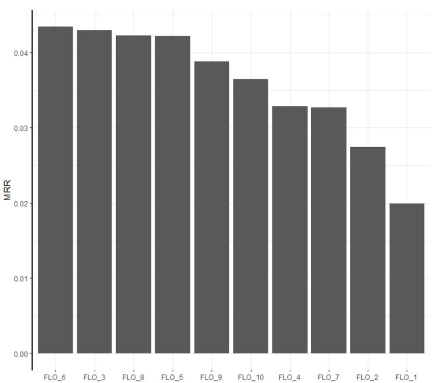
also measured the top1 accuracy, i.e. the percentage of well predicted occurrencespecies by the model at the first prediction rank. The validation performance of each model is given in tables 1 and 2. The best model is the CNN. It achieves a pretty good MRR of 0.10 knowing that the ideal MRR cannot exceed 0.409 (due to the fact that several outputs exist for the same entry). On average, it returns the correct species in the position with a success rate close to 1/20 (knowing that there is 3336 species in the training set). Nevertheless, the other models achieve good results too, all are over 0.06 of MRR and the random forest reaches almost 0.08. They return the good species label between 1 time out of 40 and 1 time out of 30. These results show that some fairly simple models can capture a strong information. It would be interesting to study the complementarity between these methods and the CNN to produce a highly predictive model. 4.2 GeoLifeCLEF challenge: submitted runs and results Fig. 2. MRR achieved by the 10 runs we submitted to the GeoLifeCLEF 2018 challenge
rank test MRR runname          participant name
            1    0.0435     FLO 6              Floris’Tic
            2    0.0430     FLO 3              Floris’Tic
            3    0.0423     FLO 8              Floris’Tic
            4    0.0422     FLO 5              Floris’Tic
            5    0.0388     FLO 9              Floris’Tic
            6    0.0365     FLO 10             Floris’Tic
            7    0.0358     ST 16      TUC MI Stefan Taubert
            8    0.0352     ST 13      TUC MI Stefan Taubert
            9    0.0348     ST 10      TUC MI Stefan Taubert
            10 0.0344       ST 9       TUC MI Stefan Taubert
            11 0.0343       ST 12      TUC MI Stefan Taubert
            12 0.0338       ST 6       TUC MI Stefan Taubert
            13 0.0329       FLO 4              Floris’Tic
            14 0.0327       FLO 7              Floris’Tic
            15 0.0326       ST 17      TUC MI Stefan Taubert
            16 0.0274       FLO 2              Floris’Tic
            17 0.0271       ST 5       TUC MI Stefan Taubert
            18 0.0220       ST 8       TUC MI Stefan Taubert
            19 0.0199       FLO 1              Floris’Tic
            20 0.0153       ST 3       TUC MI Stefan Taubert
            21 0.0153       ST 1       TUC MI Stefan Taubert
            22 0.0144       ST 14      TUC MI Stefan Taubert
            23 0.0134       ST 7       TUC MI Stefan Taubert
            24 0.0103       ST 15      TUC MI Stefan Taubert
            25 0.0099       ST 19      TUC MI Stefan Taubert
            26 0.0096       ST 11      TUC MI Stefan Taubert
            27 0.0096       ST 18      TUC MI Stefan Taubert
            28 0.0085       ST 4       TUC MI Stefan Taubert
            29 0.0030       SSN 3             SSN CS 19
            30 0.0016       SSN 4             SSN CS 19
            31 0.0016       ST 2       TUC MI Stefan Taubert
            32 0.0013       SSN 2             SSN CS 19
            33 0.0004       SSN 1             SSN CS 19
Table 3. Overview of the results of all runs submitted to GeoLifeCLEF2018.
Submissions We submitted 10 run files to be evaluated within the LifeCLEF
2018 challenge, each run file containing the prediction of a particular method on
the whole test set. It is important to note that this evaluation was conducted
entirely in blind, i.e. we never had access to the labels of the test set.
The four first run files we submitted contained the predictions of our four
main models, i.e.:
FLO 1: The predictions of the closest-location classifier model.
FLO 2: The predictions of the co-occurrence model.
FLO 3: The predictions of the environmental CNN.
FLO 4: The predictions of the spatial random forest classifier.
The other six run files we submitted corresponded to different fusion schemes
of the four base models. Indeed, the base models being trained on different kinds
of input data, we expect that their fusion may benefit from their complementar-
ity. We used two different kinds of fusion methods:
Late fusion based on probabilities: For each test item we simply average the
prediction probabilities of the fused models and then we re-sort the predictions.
Note that we could’nt do this late fusion with the closest-location classifier as it
doesn’t output probabilities, but only species ranks. For the three other models,
we evaluated the fusion of all possible pairs and the fusion of the three models:
FLO 5: late fusion of the probabilities given by the CNN and the co-occurrences
models.
FLO 6: late fusion of the probabilities given by the CNN and the spatial ran-
dom forest models.
FLO 7: late fusion of the probabilities given by the co-occurrences and the spa-
tial random forest models.
FLO 8: late fusion of the probabilities given by the CNN, the co-occurrences
and the spatial random forest models.
Late fusion based on Borda count: Borda count is a voting system allowing
to merge ranked list of candidates. In our case, it simply consists in summing
the rank of a test item in the different run files to be fused. Two new run files
were generated using this method:
FLO 9: Borda count of the predictions given by the CNN, the co-occurrences
and the spatial random forest models
FLO 10: Borda count of the predictions given by the CNN, the spatial random
forest and the closest-location classifier
Results The results we obtained within the GeoLifeCLEF challenge are pre-
sented in table 3 (along with other participant’s runs). Figure 2 illustrates the
MRR values obtained by our runs solely. The conclusions we can draw from the
results are the following:– Supremacy of the CNN model:The results show that our run FLO 6 is the best performing model among all the evaluated systems in the chal- lenge. It corresponds to the fusion of the environmental CNN model and the spatial random forest classifier. Nevertheless, the CNN model alone obtains a very close performance (FLO 3) so that the contribution of the random forest predictions to the fused model seems to be very limited. As another evidence of the supremacy of the CNN model, all our other runs including its predictions (FLO 8, FLO 5,FLO 9,FLO 10) are above all the other runs submitted to the challenge. However, their performance is degraded compared to the CNN model alone. The second best model within our four base models seems to be the spa- tial classifier based on random forest (FLO 4). Indeed, it obtains a very fair performance considering that it only uses the spatial positions of the occurrences (which makes it very easy to implement in a real-world system). The co-occurrence model (FLO 2) obtains significantly lower performance, while the closest-location classifier, which uses only the nearest point species data, is the worst model (FLO 1). – Late fusion methods comparison: We can notice that the probabilities late fusion (FLO 8) worked better than Borda’s (FLO 9). However, our late fusions, that give the same weights to fused models predictions, never significantly outperformed the best of the fused models, especially for fusions based on the environmental CNN. Though, we can wonder if learning an unbalanced weighting, or a local weighting would increase the performance. – Final results vs. cross-validation results: Overall, the MRR values achieved by our models on the blind test set of GeoLifeCLEF are much lower than the ones obtained within our cross-validation experiments (see Tables 1 and 2). We believe that this performance loss is mainly due to the construction of the blind test set, i.e. to the fact that the occurrence of a given species in the test set does never occur at a location closer than 100 meters from the occurrences of the same species in the training set. This rule was not taken into account during our cross-validation experiments on the training set. – Species community: The co-occurrence model FLO 2 seems to general- ize better than the closest-location classifier (FLO 1), though both methods used almost the same input information which is the species of the neighbor- hood. It is likely that the neural network detect the signature of a community from its input co-occurrences. For example, the network is able to predict a common mediterranean species when it gets a rare mediterranean species as entry. Indeed, the probability of observing this same rare species near its known observation is very small, but the closest location classifier would do the error.
4.3   Conclusion and perspectives

This paper reported our participation to the GeoLifeCLEF challenge aimed at
evaluating location-based species prediction models. We compared three main
types of models: (i) a convolutional neural network trained on environmental
variables extracted around the location of interest, (ii) a purely spatial model
trained with a random forest and (iii), a co-occurrence based model aimed at
predicting the likelihood of presence of a given species thanks to the knowledge
of the presence of other species. The main conclusion of our study is that the
convolutional neural network model is the best performing model. Indeed, it
achieved the best performance of the whole GeoLifeCLEF challenge. Interest-
ingly, the combination of the CNN model with the other models did not allow
any significant improvement of the results. This is surprising in the sense that
the CNN model was trained on environmental data solely whereas the other
models focused on complementary information, i.e. the spatial location and the
species co-occurrences. This suggests that the CNN model already captured all
this information, maybe because the environmental tensor associated to each
location is sufficient to recognize this particular location. In future work, we will
attempt to better understand what information the CNN does capture from that
environmental tensors and how it could be improved according to this.

References
1. Botella, C., Bonnet, P., Joly, A.: Overview of geolifeclef 2018: location-based species
   recommendation. In: CLEF working notes 2018 (2018)
2. Christophe Botella, Alexis Joly, P.B.P.M., Munoz, F.: A deep learning approach
   to species distribution modelling. Multimedia Technologies for Environmental &
   Biodiversity Informatics (2018)
3. Ioffe, S., Szegedy, C.: Batch normalization: Accelerating deep network training by
   reducing internal covariate shift. In: International Conference on Machine Learning.
   pp. 448–456 (2015)
4. Joly, Alexis and Goëau, Hervé and Botella, Christophe, Glotin, Hervé and Bon-
   net, Pierre and Planqué, Robert and Vellinga, Willem-Pier and Müller, Henning:
   Overview of lifeclef 2018: a large-scale evaluation of species identification and rec-
   ommendation algorithms in the era of ai. In: Proceedings of CLEF 2018 (2018)
5. Nair, V., Hinton, G.E.: Rectified linear units improve restricted boltzmann ma-
   chines. In: Proceedings of the 27th international conference on machine learning
   (ICML-10). pp. 807–814 (2010)
You can also read


