An Activity-based Travel Demand Model of Switzerland Based on Choices and Constraints

An Activity-based Travel Demand Model of Switzerland Based on
 Choices and Constraints

 Short paper for hEART 2019

 Wolfgang Scherr1, Chetan Joshi2, Patrick Manser1, Nathalie Frischknecht1, Denis Métrailler1
 1
 Swiss Federal Railways (SBB), Passenger Division, Service Planning, Wylerstrasse 123, 3000 Bern, Switzerland
 2
 PTV Group, 9755 SW Barnes Road, Suite 290, Portland, OR 97225, USA

 May 27, 2019

1. Introduction
Travel demand models are used to predict traffic volumes on the infrastructure and user benefits
from new service concepts. Most travel models applied in practice today simulate aggregated travel
flows, i.e. they are of macroscopic nature. In contrast, we present a microscopic model, which sim-
ulates each traveller as an individual entity.
The model is called SIMBA MOBi. It has been developed over the past two years by SBB (Swiss
Federal Railways). As far as we know, this is one of the first microscopic models that is developed
inside a transport operating company in Europe and applied to support real world business decision
making. It is person-based, multimodal, simulating 24 hours of the average weekday (Monday
through Friday) and covers the entire country of Switzerland, urban, rural and intercity. While it is
possible to derive a parameter set also for Saturdays and Sundays, using the same model structure,
this effort has not yet been undertaken as most capacity constraints in the rail and road systems are
observed on weekdays.
SIMBA MOBi starts from a synthetic resident population of Switzerland, constructs activity plans and
travel plans for each person, balancing for each traveller both the individual preferences as well as
constraints. Preferences are represented by discrete-choice models for tour and activity frequency,
destination and mode choice. Constraints are represented in the plan adjustment and scheduling
steps, using time budgets with a rule-based approach, which assures plan integrity and consistency.
Finally, 24-hour dynamic network flows for cars and public transport are simulated using the agent-
based software MATSim. Hence, the model is microscopic through all model steps.
In this paper we focus on the travel demand module, called MOBi.plans. The population synthesis
and the agent-based traffic flow simulation are not covered in this paper.

2. Previous related work
Since the origins of computer-based travel demand models in the 1960s until today, the mainstream
of transportation planning models that are used in practice has been a macroscopic (i.e. aggregated)
approach, based on several sequential steps (see Boyce and Williams, 2015). Later, the idea of
activity-based transport models (ABM) emerged and was put into practice in the 1990s. For a

 1/13

historical review see Bowman (2009) or Rasouli and Timmermans (2014). Today there are several
approaches of ABM, who differ in their focus and in terms of how far they have advanced to be used
in real world applications. The following overview presents those ABM approaches that have influ-
enced the authors in the development of SIMBA MOBi.
The North-American school of microscopic ABMs follows an econometric approach. Important rep-
resentatives who have managed to get ABM up and running in practice for several major U.S. cities
in the 2000s, are Bowman and Ben Akiva (2001), Vovsha, Bradley et al. (2004), Bhat et al. (2004).
A comprehensive presentation of the methodology is given by Castiglione et al. (2015). We borrowed
many concepts from this school for the generation of synthetic individual day-plans for each member
of a population, using a system of discrete-choice models from the generation of tours and activities
to the choice of modes, destinations and locations.
Other mainly academic ABMs can be defined as rule-based. We have drawn ideas from the work of
Roorda et al. (2008) for plan scheduling. We found few sources regarding the implementations of
time budgets in travel demand models; a rare example is Moeckel et al. (2019), using budgets of
travel time.
Agent-based models emerged in the 2000s with a focus on large-scale and network-wide micro-
scopic traffic simulation. SIMBA MOBi applies the open source software MATSim (Horni et al., 2016),
which for over a decade has been in use to model Switzerland for research purposes (Meister et al.,
2008). MATSim connects supply and demand in a network equilibrium. In addition to route search,
agents can also reschedule time and mode choices. The MATSim software does not yet include
modules to generate daily activity plans.
An earlier practice of tour-based models (Axhausen, 1989; Fellendorf et al., 1995) has a record of
many real-world applications already in the 1990s, mainly in German-speaking countries. It was
made available as part of the commercial PTV VISUM software. The aggregated calibration meth-
odology of this approach was adapted for MOBi.plans.
Building on all the approaches mentioned above, we developed a model that is activity-based and
microscopic and at the same time responsive to socio-economic shifts and to changes in transport
supply through all model steps.

3. Methodology and structure of the model
The objective of MOBi.plans is to synthetically generate an individual daily plan for each resident of
Switzerland, as represented in the synthetic population. Each individual plan contains:
 • the permanent location of primary activities, which are work and education, i.e. workplace
 and/or educational institute
 • the desired number and kind of activities a person wishes to perform in a day
 • the pattern of how those activities are bundled in tours
 • the sequence of tours and the sequence of the activities within each tour
 • the exact geographic location where each activity will be performed
 • the mode choice for each tour or subtour
 • the duration and time of day for each desired activity

Figure 1 depicts an example of a plan with all its components.

hEART 2019 – MOBi.plans 2/13

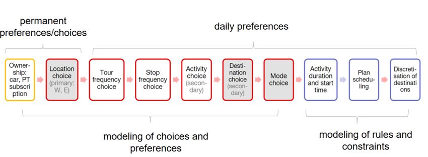
Figure 1 Example of a full-day plan with all its components

Figure 2 shows the sequence of model steps taken to construct the plans. Technical details of each
of these steps will be described later in the paper.

Figure 2 MOBi.plans model steps

3.1. Car availability and PT subscription
A first model step determines car availability and PT subscriptions (i.e. yearly or monthly public
transport passes) for each person in the population. Both are very important person attributes with
a strong impact on mode choice and destination choice. In the existing case, these attributes are
determined by choice models and then corrected based on small-area control variables (Danalet
and Mathys 2018). For the application of the model in forecasting, it is planned to integrate accessi-
bility measures for the prediction of mode availability.

hEART 2019 – MOBi.plans 3/13

3.2. Location choice
Location choice assigns permanent locations (work place and/or school place) to each person who
is in a status of employment or education. Being responsive to changes in level of service (LOS) is
a crucial requirement of the model. This is achieved with a nested model structure, where the logsum
(or maximum expected utility) of trip-based mode choice informs location choice about the service
quality of all modes to each location. Additional additive utility terms (shadow prices) in the higher
level of the location choice explain regional preferences which cannot be explained alone by physical
attributes of travel or LOS measures. The LOGIT formula of location choice is identical to the one
used in destination choice see (3.4).

3.3. Tour and activity generation
The estimation of the number of activities per person and how these activities are bundled into tours
follows the American approach of discrete-choice-based ABM as described in Bowman and Ben
Akiva (2001) and Castiglione et al. (2015). It involves discrete choice models for tour frequency,
subtour frequency and stop frequency.
A tour is defined as a sequence of trips that begin at home and end there again. Our model does not
allow for ending a tour at location different from home. Four different types of tours are modelled,
the first two being considered primary tours and the latter two secondary:

 - Work tour
 - Education tour
 - Business tour
 - Other tour

Work and education are primary activities. Both work and education are related to permanent loca-
tions and considered the dominant activity in their respective tours. On a tour, there will be additional
intermediate stops for secondary activities. Our model uses the following secondary activity types:

 - Leisure (L)
 - Shopping (S)
 - Business (B)
 - Education as non-primary activity (EC)
 - Accompany (A)
 - Other (O)

An overview of the tour and stop frequency models is shown in Table 1.
All these models are multinomial LOGITs. The perhaps most important property of the generation
models is their ability to forecast changes in the mobility of individuals in reaction to mode availability,
to changes in transport supply (by means of accessibility) and to demographic shifts (e.g. by means
of the age variable). As an example, Table 2 shows the LOGIT utility parameters of tour frequency
for “other tours” (tours without primary activity). Age and employment level are included as piece-
wise-linear variables, without a base (or “dummy”) variable. For employment there is an additional
dummy variable (employment level =0), which has special meaning: being “true” when someone is
unemployed and zero else.

hEART 2019 – MOBi.plans 4/13

Table 1 Tour- and Stop Frequency Models
 Sub tour
 Tour frequency Stop frequency
 frequency

 Number of primary tours Number of secondary tours Number of stops on primary tour Number of stops
 On primary tour
 on secondary tour
 Work Education Business Other Outbound Inbound
Constant X X X X X X X X
Employment level X X X X X X X X
Main occupation is student/pupil X X X
Age X X X X X X X X
Is in management X
Presence of kids in HH (= 80%1 0.000 -0.005* -0.017*** -0.020***
 Age < 181 0.000 -0.022 -0.047* -0.038
 18

3.4. Destination and mode choice
Knowing precisely number and type of activities each agent performs in each tour, the next step is
choosing the destination of each secondary activity and the mode for each trip between activities.
For this purpose, destination probability matrices for each activity type and different demand strata
are estimated following the same method as in location choice (see 3.1).
The probability of choosing mode m on the origin-destination pair ij is:
 ( )
 ( | ) =
 ∑ ( )
The expected maximal utility (EMU) of mode choice is then:

 = {∑[ ( / )]}
 
Mode choice depends on various variables such as travel time, distance and other level of service
measures (see Table 3). To inform destination choice about the level of service of all modes, mode
choice is nested into destination, by including EMUij (the expected maximal utility of mode choice)
into the destination choice utility:
 ( | ) = (A ) + ∙ + + 
With:
 • EMUij: maximum expected utility of mode choice from i to j
 • Aj : = the socio-economic attraction of zone j
 • λj := shadow price of destination j
 • λij := shadow price of origin-destination pair ij

For calibration purposes, it is important to extend the destination utilities with shadow prices. Finally,
the probability of choosing destination j under the condition of starting in origin i is:
 ( ( | ))
 ( | ) =
 ∑ [ ( ( | ))]

Table 3 Variables used in mode choice utility Vijm
 access/egres
 travel service number of parking
mode constant (parking distance
 time frequency transfers cost
 search) time
walk x x - - - - -
bicycle x x - - - - -
PT x x x x x - x
car - driver x x x - - x x
car - passenger x x x - - x x

However, choosing the exact destination for each stop is not as straightforward as in location choice.
Since an intermediate tour stop lies between two pre-defined locations, “rubber banding” is used to
consider both trip origin and primary location (i.e. work place) in the choice of the intermediary des-
tinations. Note that at this stage of the model, there is no interaction between the destination choice
decisions of multiple tours. In some cases, this might result in unrealistically high travel time which
violates time budgets and hence plan integrity. This issue will be treated at a later model stage (see
3.6).

hEART 2019 – MOBi.plans 6/13

3.5. Desired activity duration and activity start times
In a similar approach to the one taken by Hörl (2017), activity durations and desired activity start
times are determined based on probability distributions that were derived from the travel diary sur-
vey. The distributions distinguish several demand segments that are specific to:
 • the type of activity
 • socio-economic attributes of the person
 • the frequency of an activity in one plan (e.g. the workplace is visited once or twice)

Figure 3 Examples of probability distributions of desired activity duration

 1.0

 0.9

 0.8

 0.7

 0.6
 full time employees with 1 W-tour
 0.5
 full time employees with 2 W-tours
 0.4
 part time >40% employees with 1 W-tour
 0.3
 part time >40% employees with 2 W-tours
 0.2 part time

1. All activities must start between 0:00 and 24:00 hours (apart from the last home activity).
 2. An agent can perform only one activity or one trip at a time.
 3. The total of travel time shall not exceed the time budget X.
 4. The total of activity time shall not exceed the time budget Y.
 5. The total time spent on activity and travel episodes shall not exceed the total time budget Z,
 with Z = X + Y.

While constraints 1 and 2 will be enforced in the scheduling step (section 3.7), the step of plan
adjustment will ensure that constraints 3 through 5, i.e. the time budgets are satisfied. To satisfy time
budgets, the following changes can be performed:
 • Redo the step of activity duration choice and so modify the durations of all activities.
 • Redo the step of destination choice with the aim to obtain travel times that fit into the travel
 time budget.

We observed that 83.5% of the persons do not need an adjustment of the original preferences in
their respective plan. Of the 16.5% who need adjustment, 8.2% adjust only activity durations, while
the other 8.3% adjust also their destinations and modes. Note that the permanent locations of work
and school places are not adjusted. Only the destinations of secondary activities, which are consid-
ered day-to-day choices, are reviewed. The following figure shows a simplified view of plan adjust-
ment algorithm:

Figure 5 Rule-based plan adjustment algorithm

hEART 2019 – MOBi.plans 8/13

3.7. Scheduling procedure
The scheduling procedure takes the activity chains (and so the sequence of activities in each tour),
and the adjusted durations and travel times of all activities as they come out of step 3.6. Travel times
between activities are looked up for each individual trip as a function of travel start times. With these
inputs given, the scheduling procedure itself follows the principle of an “outward” approach described
in Castiglione et al. (2015), with the rationale that priority is given to the primary activities and their
durations, and that secondary activities and travel episodes are added before and/or after the pri-
mary activities. The procedure is given here in a simplified form:

 Order the activity chains according to priorities
 Repeat min. m and max. n times:
 For all tours:
 “Step 1”:
 Choose start time for the primary activity (or main activity)
 Block time slots needed for the duration of primary activity
 “Step 2”:
 Block time slots needed for travel times to/from secondary activities
 Block time slots needed for duration of secondary activities
 Between tours, block a minimum of 30 minutes for the home activity
 Compute objective function depending on time-of-day probability distributions
 Keep schedule if it has a higher objective value than previous best schedule
 If reached m and all activities start between 0:00 and 24:00: break
 Else: continue
 If not succeeded (exceeded n): discard the lowest tours in the priority order.
 “Step 3”: assign all remaining time slots to the home activity”

The above algorithm will discard tours from the schedule, if they do not fit into the 24 hours of the
day. This is the last resort to assure integrity of the plans. But these cases are extremely rare (less
than 4 ‰ of all trips), thanks to the step of plan adjustment (3.6), which is quite effective to assure
that the timing constraints can be met by the scheduling procedure.
Figure 6 Example of the rule-based plan scheduling

 time of day [h]
 0 1 2 3 4 5 6 7 8 9 10 11 12 13 14 15 16 17 18 19 20 21 22 23
 step 0

 step 1 work

 step 2 work L

 step 1 work L L

 step 2 work L L

 step 3 home work L L home

 Legend: home activity out-of-home activities travel

hEART 2019 – MOBi.plans 9/13

Figure 6 above illustrates the scheduling procedure for the example that was given at the introduction
of the paper in Figure 1. This particular agent obtains a day schedule packed with activities and
travel and spends only a short time at home between his/her two tours. It is a realistic plan, not
untypical for younger “singles”, who have less motivation to spend time at home during the day than
people in larger families would have.

3.8. Spatial discretisation
After the scheduling step, all plans are precise in time. Start and end times of activities and travel
times are given in hours, minutes and seconds of clock time. The spatial precision however is still
mixed at this time. While home locations have precise coordinates, locations of primary and second-
ary activities are still based on the 8000 zones that were used in location and destination choice.
In the final step of the demand model, the activity locations are broken down from zones to geo-
graphically precise coordinates. The synthetic population provides facilities, which can be busi-
nesses, other institutions or households. These facilities are precisely geo-coded. The discretisation
step choses randomly for each activity of each agent one facility among all facilities in the destina-
tion-zone that are open for the respective activity. The random draw respects weights which corre-
spond to the attractions Aj in destination choice: e.g. number of jobs in a work facility for activity work,
school enrolment for education, number of jobs in retail for shopping.
We feel that this discretisation method is very effective for our model: The zonal system, which was
defined by the Swiss Federal Government for travel modelling purposes, has a fine granularity with
in average 1000 inhabitants. In urban areas, zones are small and accessibility to the transport net-
work is homogenous across the zone, and hence random distribution of destinations can be inde-
pendent of mode availability. In rural zones with less density however, there are significant differ-
ences of accessibility between the facilities within one zone. E.g. destinations can be 50m or 2000m
from the next public transport stop. But, land use policies in Switzerland require facilities to be con-
centrated “in the village”, which is realistically represented in our synthetic population, and public
transportation stops are also always located in the village center. Still, some agent’s plans who have
chosen public transportation will obtain a destination of the trip that is not suitable for this mode. In
that case, mode choice will be corrected during agent-based traffic flow simulation (see 3.10).

3.9. Complementary exogenous travel demand
The activity-based demand model covers the travel of the resident population of Switzerland. To
produce comprehensive traffic on the networks, exogenous demand is developed from the best
available sources. The exogenous demand includes international rail travel, border crossing road
traffic, airport travel by non-residents, travel by tourists and visitors (both road and rail).

3.10. Agent-based network simulation
Endogenous plus exogenous demand is fed into an agent-based network simulation with MATSim,
which implements a spatially fully disaggregate multimodal assignment (Horni et al. 2016). The traffic
flow simulation is not described in this paper, having been calibrated earlier (Scherr et al. 2018,
Rieser et al. 2018). The use of agent-based simulation requires strong plan integrity in space and
time, as stated also in Vovsha et al. 2016. We have achieved this integrity of plans with the sched-
uling algorithm described in sections 3.6 and 3.7.
From the agent-based network model we also derive LOS-indicators, which are computed from/to
discrete locations and then aggregated from/to zones to become input of MOBi.plans.

hEART 2019 – MOBi.plans 10/13

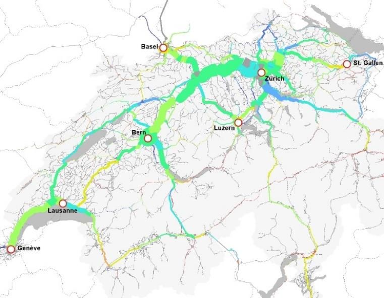
During the agent-based flow simulation in MATSim, each traveller will not only optimize route choice.
Based on his/her individually experienced network conditions, also mode choice, activity duration,
and departure time are adjusted.

4. Results and conclusions
In May 2019, the model calibration was completed for the existing state. At the time of the confer-
ence, a set of first pilot applications and sensitivity tests will be completed, and the experience will
be presented.

4.1. Validation
The model is validated in comparison to comprehensive travel statistics that include the national
travel diary survey, national rail OD-survey, rail counts, other public transportation counts, road traffic
counts, and SBB corporate data. In the following Figure 7 we show a few examples of validation.
Figure 7 Examples of model validation

 Total out-of-home time per capita Time of day distribution of travel

 Boarding & alighting at rail stations Passenger volumes, rail network

hEART 2019 – MOBi.plans 11/13

4.2. Summary: main properties of the model
The properties of the model SIMBA MOBi can be summarized as follows:
 • Activity-based approach
 • Microscopic simulation through all model steps: from generation to network flow simulation
 • High resolution of time and space
 • Use of aggregated zones in intermediary steps, while the final demand has exact geographic
 locations for all destinations in a plan
 • Person-based simulation, taking household properties in consideration in persons’ decisions,
 but not modelling household interactions explicitly.
 • Representation of 24 hours of the average weekday
 • Strong integrity of the time and space sequence of activities and travel along 24-hour plans
 • A focus on the representation of variables (person attributes and transport LOS) that explain
 travel choice for or against public transportation.
 • A strong effort in model calibration to allow for the analysis of travel volumes and capacities
 on a transportation project level.

4.3. Conclusions
Based on our experience we state that microscopic activity-based models are ready for practice. We
have achieved model calibration to a goodness of fit as it is expected in the practice of macroscopic
models. Microscopic models today require more staff time and computer resources than conven-
tional models. Some of the reasons are: complexity of the approach, increased amount of data and
parameters, software tools still being under development in terms of functionality and user friendli-
ness. We continue to work on improving usability and computational efficiency. On the other hand,
there is a lot of benefit from microscopic modeling. The high geographic and socio-economic gran-
ularity of travel demand allows for analyses that were unthinkable with conventional models. Among
those are: traveler composition according to multiple attributes, coverage of all legs of travel from
door to door, time-dynamic outputs over 24-hours, analysis of all public transportation stops without
the limitation to major stations. Further, we expect increased possibilities in forecasting future mobil-
ities: Agent-based traffic flow simulation enables the integration of new travel modes and the activity-
based demand model allows for changes in activity and travel patterns of future populations (e.g.
“active seniors” perform more activities and longer trips than the same age group does today.

hEART 2019 – MOBi.plans 12/13

5. References
Axhausen, K.W.: (1989): Simulating activity chains. German approach. Journal of transportation en-
gineering, 115 (3) 316-325.
Bhat, C.R., J.Y. Guo, S. Srinivasan, A. Sivakumar (2004): Comprehensive Econometric Microsimu-
lator for Daily Activity-Travel Patterns. Transportation Research Record, Vol. 1894, p. 57-66.
Bierlaire, M. (2016) PythonBiogeme: a short introduction. Report TRANSP-OR 160706. Series on
Biogeme. Transport and Mobility Laboratory, School of Architecture, Civil and Environmental Engi-
neering, Ecole Polytechnique Fédérale de Lausanne, Switzerland.
Bowman, J. L. and M. E. Ben-Akiva (2001) Activity-based disaggregate travel demand model system
with activity schedules, Transportation Research Part A, 35(2001), p. 1-28.
Bowman, J. L. (2009): Historical Development of Activity Based Model Theory and Practice, Traffic
Engineering and Control, Vol. 50, No. 2: 59-62 (part 1), No. 7: 314-318 (part 2).
Boyce, D., H. Williams (2015): Forecasting Urban Travel: Past, Present and Future. Cheltenham,
U.K. and Northampton, Mass.
Castiglione, J., Bradley, M., Gliebe, J. (2015): Activity-Based Travel Demand Models: A Primer.
SHRP 2 Report S2-C46-RR-1. Transportation research Board (TRB), Washington, D.C.
Danalet, A. and N. Mathys (2018): Mobility resources in Switzerland 2015. Conference paper, STRC
2018, Ascona, Switzerland.
Federal Statistical Office (2017): Population's transport behavior 2015. Key results of the mobility
and transport microcensus. Bundesamt for Statistik (BfS, Federal Statistical Office), Neuchâtel, Swit-
zerland.
Fellendorf, M., Haupt, T., Heidl, U., Scherr, W. (1997): PTV Vision: Activity-Based Demand Fore-
casting in Daily Practice. In: D.F. Ettema, H.J. Timmermans (Ed.): Activity-Based Approaches to
Travel Analysis, Elsevier, Oxford / New York, 1997, p. 55-72.
Horni, A., Nagel, K., Axhausen, K. (2016): The Multi-Agent Transport Simulation MATSim. London.
Meister, K., Rieser, M., Ciari, F., Horni, A., Balmer, M., Axhausen, K. (2008): Anwendung eines
agentenbasierten Modells der Verkehrsnachfrage auf die Schweiz. Conference paper, Heureka,
Stuttgart, Germany.
Moeckel, R., Kuehnel, N., Llorca, C. and Moreno, A. (2019): Agent-Based Travel Demand Modeling:
Agility of an Advanced Disaggregate Trip-Based Model. Conference Paper, presented at the TRB
Annual Meeting, Washington, D.C.
Rasouli, S. and Timmermans, H. (2014): Activity-based models of travel demand: promises, pro-
gress and prospects. International Journal of Urban Sciences. Vol. 18, No. 1, 30-60. Abington, U.K.
Rieser, M., Métrailler, D., Lieberherr, J. (2018): Adding realism and efficiency to public transportation
in MATSim. Proceedings of the Swiss Transportation Research Conference, Ascona, Switzerland.
Roorda, M.J. Miller, E.J., Habib, K.M.N. (2008): Validation of TASHA: A 24-hour activity scheduling
microsimulation model. Transportation Research Part A, 42 (2008), p. 360–375
Scherr, W., Bützberger, P., Frischknecht, N. (2018): Micro Meets Macro: A Transport Model Archi-
tecture Aiming at Forecasting a Passenger Railway's Future. Proceedings of the Swiss Transporta-
tion Research Conference, Ascona, Switzerland.
Vovsha, P., Anderson, R, Giamo, G., Rousseau, G. (2016): Integrated Model of Travel Demand and
Network Simulation. Conference paper ITM 2016, Denver.
Vovsha, P., Bradley, M., Bowman, J. (2004): Activity-based travel forecasting models in the United
States: Progress since 1995 and Prospects for the Future. Paper for presentation at the EIRASS
Conference on Progress in Activity-Based Analysis, Maastricht, The Netherlands.

hEART 2019 – MOBi.plans 13/13