Dosimetry of Various Human Bodies Exposed to Microwave Broadband Electromagnetic Pulses
←
→
Page content transcription
If your browser does not render page correctly, please read the page content below
ORIGINAL RESEARCH
                                                                                                                                             published: 13 August 2021
                                                                                                                                      doi: 10.3389/fpubh.2021.725310

                                              Dosimetry of Various Human Bodies
                                              Exposed to Microwave Broadband
                                              Electromagnetic Pulses
                                              Jerdvisanop Chakarothai*, Kanako Wake and Katsumi Fujii

                                              Electromagnetic Compatibility Laboratory, Electromagnetic Standards Research Center, Radio Research Institute, National
                                              Institute of Information and Communications Technology, Koganei, Japan

                                              In this paper, human exposures to ultra-wideband (UWB) electromagnetic (EM) pulses
                                              in the microwave region are assessed using a frequency-dependent FDTD scheme
                                              previously proposed by the authors. Complex permittivity functions of all biological
                                              tissues used in the numerical analyses are accurately expressed by the four-term
                                              Cole–Cole model. In our method, we apply the fast inverse Laplace transform to
                                              determine the time-domain impulse response, utilize the Prony method to find the
                                              Z-domain representation, and extract residues and poles for use in the FDTD formulation.
                                              Update equations for the electric field are then derived via the Z-transformation. Firstly,
                                              we perform reflection and transmission analyses of a multilayer composed of six different
                                              biological tissues and then confirm the validity of the proposed method by comparison
                         Edited by:
                                              with analytical results. Finally, numerical dosimetry of various human bodies exposed
                      Tongning Wu,
   China Academy of Information and           to EM pulses from the front in the microwave frequency range is performed, and
  Communications Technology, China            the specific energy absorption is evaluated and compared with that prescribed in
                       Reviewed by:           international guidelines.
                        Yinliang Diao,
Nagoya Institute of Technology, Japan         Keywords: electromagnetic pulses, finite-difference time-domain method, fast inverse Laplace transform, Prony
                       Congsheng Li,          method, exposure assessment
  China Academy of Information and
 Communications Technology, China

                  *Correspondence:            INTRODUCTION
              Jerdvisanop Chakarothai
                       jerd@nict.go.jp        In 2002, the Federal Communications Commission of the United States of America issued a ruling
                                              allowing the use of ultra-wideband (UWB) electromagnetic (EM) pulses in the frequency range
                    Specialty section:        between 3.1 and 10.6 GHz (1). Since then, numerous applications of UWB pulses have emerged as
          This article was submitted to       a result of the regulation, such as vital signal detection and locating moving human bodies, as well
                  Radiation and Health,       as ground-penetrating radar, remote sensing, non-destructive inspection, and so forth (2). Owing
                a section of the journal
                                              to many advantages of UWB pulses such as low power consumption and immunity to multipath of
              Frontiers in Public Health
                                              EM propagations and EM interferences, the widespread use of EM pulses is expected to continue.
            Received: 15 June 2021            Some of these applications use UWB pulses in the vicinity of human bodies, such as wireless capsule
            Accepted: 21 July 2021
                                              endoscopy using broadband EM pulses for on/in-body communications (3, 4). These applications
          Published: 13 August 2021
                                              have led to public concern about the effect on the broadband EM pulses to human body.
                             Citation:
                                                  Meanwhile, biological effects due to EM pulses have been numerically and experimentally
    Chakarothai J, Wake K and Fujii K
  (2021) Dosimetry of Various Human
                                              investigated. The effects include the microwave hearing effect, microwave heating effect, and
       Bodies Exposed to Microwave            electroporation (5–9). Consequently, international organizations have prescribed exposure limits
  Broadband Electromagnetic Pulses.           for the temporal peak of specific energy absorption (SA) in published guidelines to prevent adverse
       Front. Public Health 9:725310.         effects, particularly of microwave hearing, which is considered an acute biological effect (10, 11).
    doi: 10.3389/fpubh.2021.725310            The International Commission on Non-ionizing Radio Protection (ICNIRP) provided an SA limit

Frontiers in Public Health | www.frontiersin.org                                    1                                          August 2021 | Volume 9 | Article 725310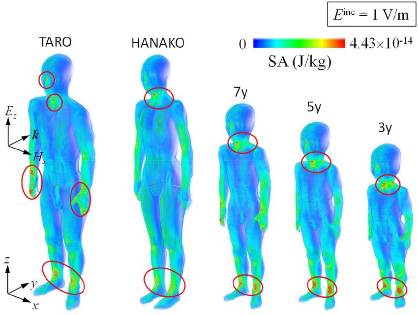
Chakarothai et al.                                                                                            Human Body Exposures by EM Pulses

of 2 mJ/kg in an arbitrary 10 g-averaged tissue for a single               functions in the complex frequency domain to transform them
pulse illumination (10), while the SA limit is up to 576 J/kg              into time-domain impulse responses. Then, the Prony method
for continuous exposure of 6 min in the regulation defined by              is used to extract the model parameters and to determine
the Institute of Electrical and Electronics Engineers (IEEE) (11).         expressions for the infinite impulse response (IIR) expressions in
Recently, the ICNIRP has revised the Guidelines based on the               the Z-domain. The update equations of electric field are derived
relevant scientific knowledge and published them in 2020. In               via the Z-transform.
the guidelines, it is mentioned that there is no evidence that                This paper is outlined as follows. The proposed (FD)2 TD
microwave hearing in any realistic exposure scenarios causes               formulation and the calculation of the update coefficients for
adverse health consequence and the microwave hearing effect is             the electric field are described in section (FD)2 TD Formulation
not considered in the guideline but it is still mandate to consider        Using FILT and Prony Method. The validity of the method in
the heating effect from the pulse exposures (12). Although many            calculating SA and internal electric field strength (IEFS) inside
biological effects due to EM pulses have been experimentally               a multilayer model of biological tissues is demonstrated via
confirmed, there are few studies providing detailed exposure               comparison with the theoretical results in section Transmission
levels or showing the distribution of SA inside a human body.              Characteristics of EM Pulses Into Biological Bodies. Numerical
   To derive SA inside the human body, calculation of                      dosimetry of anatomically detailed human body models exposed
the interactions between EM pulses and biological bodies is                to UWB EM pulses is performed and physical quantities such
necessary. In the earliest studies, most of the biological targets         as SA and IEFS are quantitatively derived and compared with
were objects having simple shapes such as a multilayer or a                those prescribed in the guidelines in section Transmission
dielectric sphere, inside which SA or the induced electric field           Characteristics of EM Pulses Into Biological Bodies. Finally,
was derived theoretically (13, 14). However, there has been no             conclusions are drawn in section Conclusion.
detailed dosimetric information of the detailed human body
exposed to EM pulses due to difficulties in the calculation of             (FD)2 TD FORMULATION USING FILT AND
SA or the induced electric field inside biological bodies. These
problems are mainly attributed to the frequency dependence of
                                                                           PRONY METHOD
the dielectric properties of biological tissues, which are expressed       Methodology
by the four-term Cole-Cole model (15).                                     In this study, all media used in the numerical analyses are
   To perform numerical dosimetry of EM pulses, we need                    biological tissues having complex relative permittivity expressed
to consider the frequency dependence of the permittivity                   by the four-term Cole–Cole function as
and conductivity of biological tissues over a broad frequency
range. Many frequency-dependent finite-difference time-domain                                                 4
                                                                                                                    1χq
                                                                                                      σ     X
[(FD)2 TD] approaches have been proposed, such as recursive                         εm (ω) = ε∞ +         +              1−αq ,               (1)
                                                                                                     jωε0
convolution method (16), piecewise linear recursive convolution                                             q=1 1 + jωτq
method (17), trapezoidal recursive convolution method (18),
auxiliary differential equation method (19–21), and Z-transform            where, ω, ε∞ , and σ are the angular frequency [rad/s], relative
method (22). However, these approaches have only been applied              permittivity and conductivity [S/m] of a biological medium at
to materials having complex permittivity expressed by relatively           infinite frequency, respectively. ε0 is the free-space permittivity
simple models such as the Debye and Lorentz models. These                  and 1χq represents the change in relative permittivity in
approaches are not applicable to the Cole–Cole function, due               the qth relaxation term. τq and αq are the relaxation time
to difficulties in finding the exact time-domain solution of               and a parameter determining the broadness of the qth term,
a fractional-order differential equation. Nevertheless, many               respectively. All parameters in (1) can be found in Gabriel’s
attempts have been made to address this problem, including                 database of dielectric properties for biological tissues (15).
those using the Riemann–Liouville theory to find the time-                 Although Gabriel’s permittivity data are de facto, it is noteworthy
domain solution of the model (23, 24). Recently, our research              that different Cole–Cole parameters may be derived, depending
group has proposed an FDTD formulation for analyses of                     on the method used in fitting the measurement data of the
arbitrary frequency-dependent materials via the use of the                 dielectric properties. By limiting the frequency range to between
fast inverse Laplace transform (FILT) and the Prony method                 1 MHz and 20 GHz, the number of Cole–Cole terms may be
(25). The proposed method has also been extended to three-                 reduced from four terms to two terms while providing the best
dimensional analyses of UWB antennas in the vicinity of the                fit to the measurement data (28). The average deviations from
human body and the dosimetry of EM pulses incident to a human              the measurement results over a frequency range between 1 MHz
head (26, 27).                                                             and 20 GHz are higher than 20% for both relative permittivity
   In this study, we extend our numerical models to whole-                 and loss factor of some biological tissues but they are shown to be
body human models which are exposed to broadband EM pulses.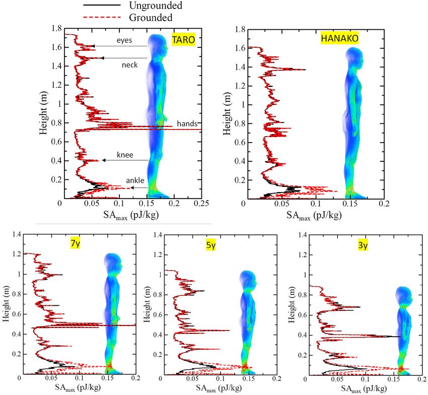
Chakarothai et al. Human Body Exposures by EM Pulses
the relaxation time normalized by the time step interval used in Calculation of Specific Energy Absorption
the FDTD simulations and obtain impulse responses for each and Internal Electric Field Strength
susceptibility term in the time domain. Then, we use the Prony The exposure level inside biological bodies illuminated by
method to transform the time-domain impulse response into broadband EM pulses can be evaluated using SA, which has been
that in the Z-domain. The permittivity is now expressed in the used as a metric in the guidelines. In the FDTD simulations, SA
Z-domain as can be calculated using the following equation:
4 Lq (q) n
1 + z−1 σ 1t X X Al
1 X E (t) ∂D (t)
εm (z) = ε∞ + −1
+ (q)
, (2) SAn− 2 = 1t · ,
1−z 2ε0 1 − p z−1 ρ ∂t t= m− 12 1t
q=1 l=1 l m=1
n
1 X
where 1t and Lq are the time step interval and number of poles Em +Em−1 · Dm −Dm−1 ,
= (8)
(q) (q) 2ρ
for the qth Cole–Cole term, respectively. Al and pl are residues m=1
and poles, respectively. Note that the second term of the right
where ρ is the density of the biological tissue. The electric flux
hand side is obtained by applying the bilinear approximation,
density in Equation (7) at the nth time step (Dn ) is updated using
i.e., jω ≈ s = 2 1 − z−1 / 1 + z−1 / (1t). Since the nested
the magnetic field at the (n+1/2)th time step (Hn+1/2 ) and En is
summation in the third term of the right-hand side of (2) can be
updated using (4).
merged into a single summation, (2) can simply be expressed as
Since a broadband pulse is utilized in our simulations, we can
N also obtain numerical solutions of the electric and magnetic fields
1 + z−1 σ 1t X Ak at each frequency component within a single run. The electric
εm (z) = ε∞ + −1
+ , (3)
1−z 2ε0 1 − pk z−1 field at a frequency is determined via Fourier transform of the
k=1
waveform obtained at an observation location as
where N is the total number of Debye terms, i.e., N = L1 +
NT
L2 + L3 + L4 . Procedures for determining N, Ak , and pk using Z T X
the Prony method will be described in subsection Calculation of E (ω) = E (t) e −jωt
dt= En e−jωn1t 1t, (9)
0 n=0
Specific Energy Absorption and Internal Electric Field Strength
and can also be found in the literature (25). Substituting (3) into
the discrete constitutional relation of Maxwell’s equations, we where N T is the total number of time steps. After the electric field
obtain the update equation for the electric field as at each frequency is obtained, the specific absorption rate (SAR)
is then calculated as follows:
N
" #
n1 Dn σ 1t n−1 n−1
X
n−1 σ |E (ω)|2
E = − E −I − pk Pk , (4) SAR (ω) = . (10)
L0 ε0 2ε0 2ρ
k=1
where, Calculation of Update Coefficients for
N
Electric Field
σ 1t X The procedures for determining coefficients Ak and pk in the
L0 = ε∞ + + Ak (5)
2ε0 update equation for the electric field are described as follows.
k=1
First, we transform relative permittivity represented in the
n n−1 σ 1t n
E + En−1 frequency domain into that in the complex frequency domain by
I = I + (6)
2ε0 replacing jω with the complex frequency s and apply the FILT
Pnk = pk Pn−1
k + Ak En , (7) to find impulse response of the permittivity in the time domain.
Then, the Prony method is used to extract the residues Ak and
In and Pnk are the auxiliary variables which are initialized by poles pk from the expression for the IIR in the Z-domain.
setting I0 = 0 and P0k = 0, respectively. Equations (4), (6), and As an example, we apply the FILT and the Prony method to
(7) are the update equations for the electric field, the auxiliary the permittivity functions of biological tissues “Fat” and “Gray
field used for considering the conductivity term, and the auxiliary Matter.” Each Cole–Cole parameter is taken from the Gabriel’s
field used for considering the Cole–Cole terms, respectively. database and listed in Table 1. The time step interval 1t used to
The update equations for the electric flux density and magnetic normalize the relaxation time in the Cole–Cole function before
field can be obtained by applying the central difference to applying the FILT is set to 1.668 ps.
Maxwell’s equations similarly to those in conventional FDTD Table 2 shows the update coefficients Ak and pk used in the
procedures (20). FDTD calculations for “Fat” and “Gray Matter.” These values
The main advantages of the proposed method are that are directly obtained from the Prony method and the number of
we can avoid the formulation of fractional-order differential coefficients for each Cole–Cole term is truncated when the ratio
equations by using the FILT and the Prony method and it is of {|Ak | / max |Ak |} for k = 1, 2, . . . , N is less than a tolerance
straightforward to implement the proposed method into the value of 10−3 . The update coefficients Ak and pk physically
conventional FDTD code. correspond to the initial amplitude and the decreasing ratio of
Frontiers in Public Health | www.frontiersin.org 3 August 2021 | Volume 9 | Article 725310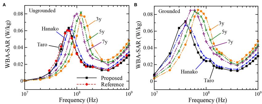
Chakarothai et al.                                                                                                                       Human Body Exposures by EM Pulses

TABLE 1 | Cole–Cole parameters for “Fat” and “Gray Matter” from Gabriel’s database.

Tissue name                ε∞                  σ (S/m)                     1st term                   2nd term                      3rd term                        4th term

Fat                        2.5                 0.035                        1χ1 = 9                   1χ2 = 35                  1χ3 = 3.3 × 10⁴                  1χ4 = 107
                                                                         τ1 = 7.958 ps             τ2 = 15.915 ns               τ3 = 159.155 ms                  τ4 = 15.915 ms
                                                                            α1 = 0.2                  α2 = 0.1                     α3 = 0.05                        α4 = 0.01
Gray Matter                 4                   0.02                       1χ1 = 45                  1χ2 = 400                  1χ3 = 2.0 × 10⁵                  1χ4 =4.5 × 10⁷
                                                                         τ1 = 7.958 ps             τ2 = 15.915 ns               τ3 = 106.103 ms                  τ4 = 5.305 ms
                                                                            α1 = 0.1                  α2 = 0.15                    α3 = 0.22                          α4 = 0

TABLE 2 | Update coefficients for “Fat” and “Gray Matter.”

Cole-Cole                    Fat                                    Gray Matter
terms
                     Ak                   pk                   Ak                 pk

1st           A1   = 0.51370       p1   = 0.82495      A1    = 3.94634     p1 = 0.80579
              A2   = 0.44668       p2   = 0.71195      A2    = 2.27434     p2 = 0.69670
              A3   = 0.38560       p3   = 0.54623      A3    = 1.16025     p3 = 0.88246
              A4   = 0.27620       p4   = 0.90559      A4    = 1.01923     p4 = 0.51558
              A5   = 0.18682       p5   = 0.33125      A5    = 0.57702     p5 = 0.29143
              A6   = 0.16287       p6   = 0.96186      A6    = 0.12362     p6 = 0.95064
              A7   = 0.02939       p7   = 0.11328      A7    = 0.32517     p7 = 0.09047
              A8   = 0.00263       p8   = 0.99134      A8    = 0.00886      p8 = 0.98824
2nd           A9 = 0.00456       p9 = 0.99981          A9 = 0.05766        p9 = 0.99977
              A10 = 0.00137      p10 = 0.99470         A10 = 0.02718       p10 = 0.99451
              A11 = 0.00090      p11 = 0.96716         A11 = 0.01975       p11 = 0.96773
              A12 = 0.00067      p12 = 0.89813         A12 = 0.01582       p12 = 0.90147
              A13 = 0.00054      p13 = 0.77398         A13 = 0.01333       p13 = 0.78223
                                                       A14 = 0.01158       p14 = 0.60236
                                                       A15 = 0.00997       p15 = 0.36732
                                                       A16 = 0.00762       p16 = 0.12557
3rd           A14 = 0.00060      p14 = 0.99998         A17   = 0.03134     p17 = 0.99991        FIGURE 1 | Reflection coefficients of “Fat” and “Gray Matter”.
                                                       A18   = 0.01880     p18 = 0.99735
                                                       A19   = 0.01668     p19 = 0.98646
                                                       A20   = 0.01495     p20 = 0.96009
                                                       A21   = 0.01353     p21 = 0.91205          As shown in Figure 1, the reflection coefficients of “Fat” and
                                                       A22   = 0.01233     p22 = 0.83801
                                                                                               “Gray Matter” obtained via numerical simulations are within
                                                       A23   = 0.01125     p23 = 0.73622
                                                       A24   = 0.01025     p24 = 0.60828       2% of those obtained by the analytical method over a broad
                                                       A25   = 0.00926     p25 = 0.46002       frequency range between 50 MHz and 10 GHz, demonstrating the
                                                       A26   = 0.00820     p26 = 0.30292       validity of the update coefficients and our numerical approach.
                                                       A27   = 0.00694     p27 = 0.15589       Update coefficients for the other type of biological tissues can also
                                                       A28   = 0.00533     p28 = 0.04538
                                                                                               be calculated straightforwardly using the procedures described
4th           A15 = 0.00122      p15 = 1.00000         A29 = 0.01415       P29 = 1.00000
                                                                                               above. Note that when we change the time step interval, we also
                                                                                               need to recalculate the update coefficients.

the time-domain impulse response, respectively. From Table 2,                                  TRANSMISSION CHARACTERISTICS OF
the total numbers of coefficients are 15 and 29 for “Fat” and “Gray                            EM PULSES INTO BIOLOGICAL BODIES
Matter,” respectively.
    To demonstrate the validity of the update coefficients, we                                 Multilayer Model
calculate the reflection coefficients from each biological medium                              Figure 2 shows a multilayer model mimicking a human head,
by one-dimensional FDTD simulation using the model shown as                                    which comprises six biological tissues, similar to those used
Figure 4 in Chakarothai et al. (26) and compare their values with                              in the literature (29, 30). Table 3 indicates the thicknesses of
those obtained from the EM theory. The analysis model is half                                  biological tissues used in the analysis model and the number
filled with biological tissues and truncated with perfectly matched                            of the update coefficients for each biological tissue. The total
layers in order to absorb the outgoing wave. Numerical results                                 size of the multilayer model is 180 mm. These coefficients are
using a time step interval of 1.668 ps and a resolution of 0.5 mm                              obtained by applying the FILT and the Prony method with a
are shown in Figure 1. The reflection coefficients are analytically                            time step interval of 1t = 1.668 ps. The resolution and the total
                                √           √
calculated using Ŵ = 1 − εm / 1 + εm , where εm is the                                         number of cells used in our analysis model are 0.5 mm and 5,000,
complex relative permittivity expressed by Equation (1).                                       respectively. CPMLs with eight layers are utilized on both sides

Frontiers in Public Health | www.frontiersin.org                                           4                                           August 2021 | Volume 9 | Article 725310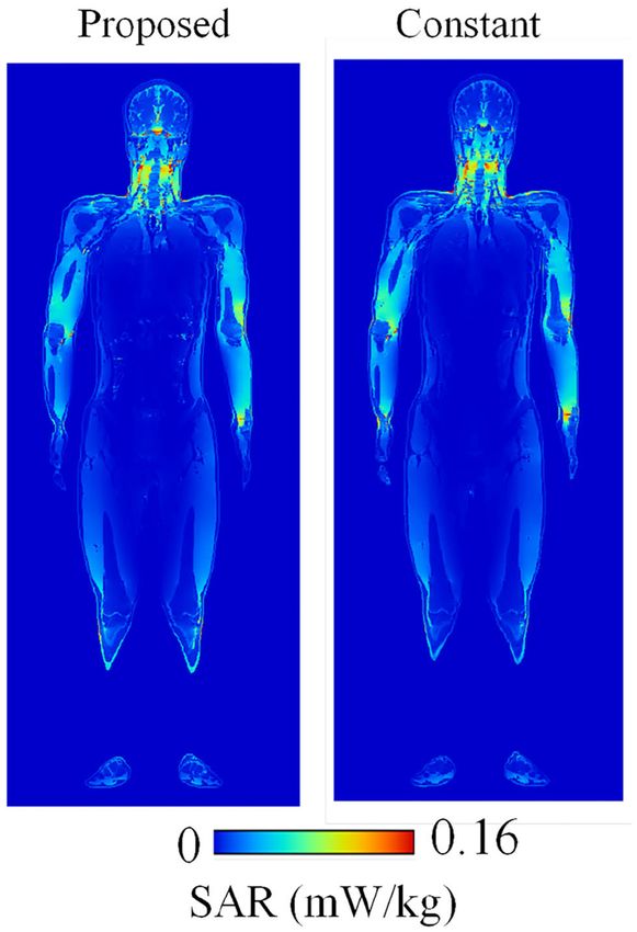
Chakarothai et al.                                                                                                               Human Body Exposures by EM Pulses

 FIGURE 2 | Multilayer model consisting of six biological tissues.

TABLE 3 | Tissue density and thickness of each tissue layer.

Tissue name                    Thickness (mm)             Number of coefficients

Skin (Wet)                        d1 = 1.0                           21
Fat                               d2 = 1.5                           15
Bone                              d3 = 4.0                           14
Dura                              d4 = 1.0                           16
CSF                               d5 = 3.0                           9
Brain (Gray Matter)               d6 = 159                           29

of the analysis domain to absorb the outgoing EM waves. The
total number of time steps is 100,000. The incident electric field
is given by a Gaussian pulse expressed as
                                                  2 !
                     inc               t − T0
                E          (t) = exp −                    u (t),           (11)         FIGURE 3 | Reflection coefficient and transmission of multilayer mimicking a
                                         a0                                             human head model.

where T 0 = 0.250 ns, a0 = 0.0633 ns, and u(t) is the unit
step function, which is applied from the air region on the
left side as shown in Figure 2. The applied Gaussian pulse                             with increasing frequency and reaches a minimum value of 0.38
contains frequency components from dc to approximately 9.3                             at ∼2 GHz, while the transmission exhibits peak at 2 GHz. From
GHz, where the power of the pulse decreases 1,000-fold from its                        Figure 3, more than 80% of the incident power penetrates into
maximum value. Number of sampling points used in fast Fourier                          the multilayer model at the maximum transmission frequency of
transform to obtain the reflection coefficients and transmission                       around 2 GHz. Note that the maximum transmission frequency
characteristics is 120,000. Zero padding is used after 100,000                         depends on the thicknesses of the biological tissues in the model;
sampling data.                                                                         thus, using a different model will yield different results from those
    Figure 3 indicates the reflection coefficient and the                              shown in this study. Next, the transmission characteristics of
transmission of the multilayer model as a percentage obtained by                       the EM pulse are obtained from the ratio between the receiving
the FDTD and analytical methods from 50 MHz to 10 GHz. The                             power at an observation point inside a biological tissue layer and
transmission, indicating the power transmitting into a biological                      the power penetrating into the model from the leftmost boundary
tissue layer, is calculated using the following equation:                              of the skin layer.
                                                                                           Figure 4 indicates the transmission characteristics at the
                      Pt (ω) = 1 − |Ŵ|2 × 100 [%] ,

                                                                           (12)        center of each layer in the left half of the analysis model as a
                                                                                       percentage. From the figure, we observe a peak of the transmitted
where Ŵ is the reflection coefficient. It is shown that the                            power in the skin at around 2.5 GHz. This peak shifts to a higher
numerical and analytical results are in good agreement,                                frequency with decreasing maximum value when the power
demonstrating the validity of our proposed FDTD method again.                          penetrates into the subsequent layer, which is the “Bone” layer
Note also that the broadband results are numerically obtained in                       in this case. It is also shown that when the observation point is
the time domain by a single FDTD run and transformed to those                          located inside the CSF layer, the transmission characteristics of
in the frequency domain via the fast Fourier transform. From                           this multilayer model are almost flat in the range between 300
the results, it can be seen that the reflection coefficient decreases                  and 800 MHz, having a maximum at ∼500 MHz. In addition,

Frontiers in Public Health | www.frontiersin.org                                   5                                           August 2021 | Volume 9 | Article 725310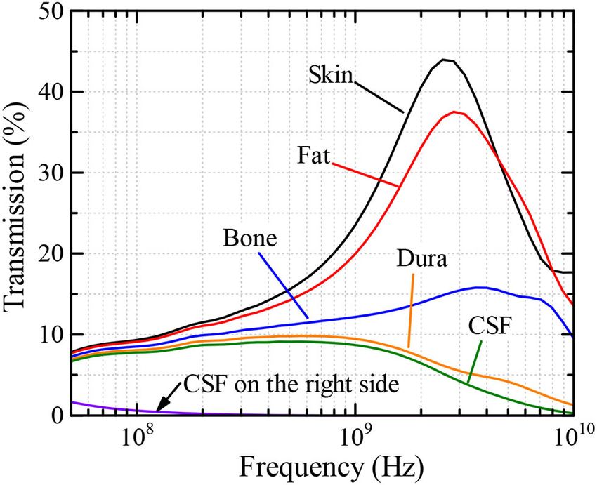
Chakarothai et al.                                                                                                             Human Body Exposures by EM Pulses

when the frequency is larger than 1 GHz, most of the power is                        with increasing frequency in this region, except between 5 and 8
absorbed at the superficial layers before reaching the CSF layer                     GHz, where the transmissions in the “Fat” layer is greater than
and, therefore, the transmitted power monotonically decreases                        that in the “Skin” layer. This may be due to a small loss in
                                                                                     the “Bone,” compared to that of “Skin,” and multiple reflections
                                                                                     occurring between the Skin–Fat and Fat–Bone boundaries that
                                                                                     create a local maximum. Note that only a small proportion of the
                                                                                     power reaches the other side of the analysis region. For example,
                                                                                     as shown in Figure 4, the transmission power that reaches the
                                                                                     CSF layer on the right side of the analysis model is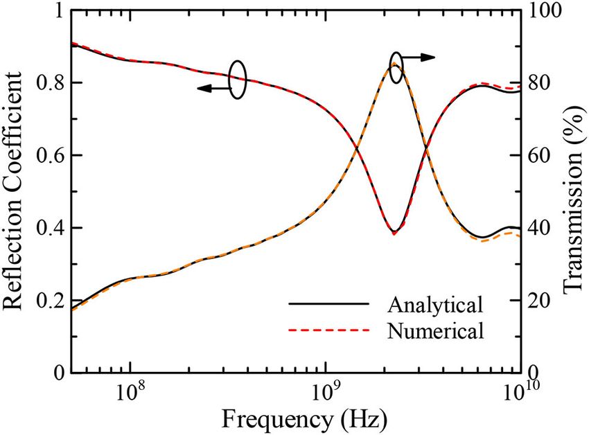
Chakarothai et al.                                                                                                       Human Body Exposures by EM Pulses

TABLE 4 | Calculation time and memory usage for each model.

Model                       Memory usage (GBytes)         Size of analysis region (cells)       Calculation time (s)          Calculation time with constant
                                                                                                                              permittivity at a frequency (s)

Male (TARO)                             88.6                    200 × 360 × 906                  45,090 (12 h 31 min)                14,767 (4 h 6 min)
Female (HANAKO)                         81.7                    200 × 360 × 844                   34,124 (9 h 29 min)                13,547 (3 h 46 min)
7-year child                            29.2                    146 × 225 × 645                   11,598 (3 h 13 min)                4,677 (1 h 18 min)
5-year child                            20.8                    136 × 196 × 560                   11,067 (3 h 4 min)                   2,942 (49 min)
3-year child                            16.6                    132 × 187 × 481                   9,126 (2 h 32 min)                   2,795 (47 min)

different biological tissues and have a spatial resolution of 2 mm.
Figure 5 also shows exposure situations with an ungrounded
model (free-space model) and a grounded model standing on
a ground plane made of the perfectly electric conductor (PEC).
The height and weight for each numerical human model are
also indicated in Figure 5. In accordance with the Courant
condition, the time step interval is determined as 3.85 ps.
The time step interval used here is different from that used
in subsection Multilayer Model; thus, we need to recalculate
the update coefficients for all biological tissues used in the
numerical simulations.
    The update coefficients are derived by applying the FILT
and the Prony method as described above. The time step
interval used to normalize the relaxation time in the Cole–
Cole function is then set to 3.85 ps, the same as that used
in the numerical simulations. After calculating the update
coefficients, we validate them by performing one-dimensional
simulations and computing the reflection coefficients. We have
found that the reflection coefficients of all biological media
having a permittivity function characterized by the Cole–Cole
model match those obtained from the EM theory with a small
difference of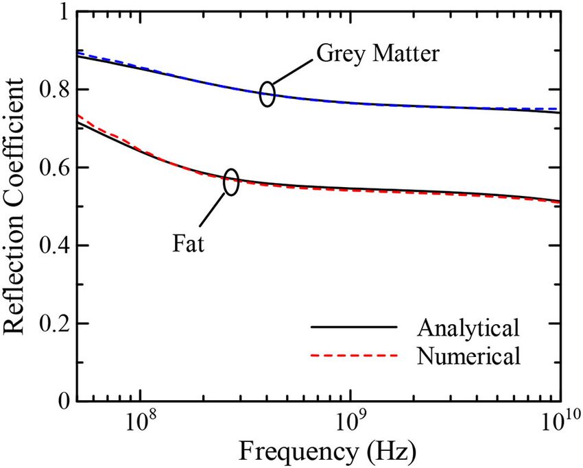
Chakarothai et al.                                                                                                   Human Body Exposures by EM Pulses

 FIGURE 7 | Whole-body average SAR over a frequency range between 10 MHz to 1 GHz, calculated using the proposed FDTD method for the ungrounded and
 grounded cases. (A) Ungrounded cases. (B) Grounded cases.

 FIGURE 8 | SA distribution for one pulse illumination for various ungrounded human models.

Frontiers in Public Health | www.frontiersin.org                                8                                   August 2021 | Volume 9 | Article 725310
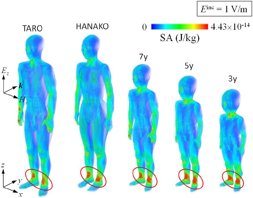
Chakarothai et al.                                                                                                   Human Body Exposures by EM Pulses

 FIGURE 9 | SA distribution for one pulse illumination for various grounded human models.

model was
Chakarothai et al.                                                                                                   Human Body Exposures by EM Pulses

 FIGURE 10 | Maximum SA at each height for various human models for 1 V/m electric field strength.

expense of using more memory. From Figure 7, the SAR peak                           forearm, and neck; SA increases by 53% (adult male) to 74%
is found at around 70 MHz for the ungrounded TARO model,                            (3-y-child) at the ankle, whereas SA at the other parts remain
which corresponds to the whole-body resonance and the peak                          almost the same in the ungrounded cases. Figure 10 shows the
frequency increases for the shorter HANAKO, 7-, 5-, and 3-y-                        layer maximum SA at each height of various human bodies when
child models. For grounded conditions, the SAR peaks occur at                       exposed to an EM pulse of 1 V/m, polarized in the z-direction.
40 and 70 MHz for the adult and 3-y-child models, respectively.                     The peak SA and the SA at the ankle for various human models,
These results are in good agreement with those indicated in the                     which are normalized to the ICNIRP-prescribed power density
literature (32, 34).                                                                limit of 2 W/m2 , are summarized in Table 5 (10). Note that the
    Figures 8, 9 show SA distributions on the human surface                         power density limit is constant for 10–400 MHz and increases
for ungrounded and grounded cases, respectively. For the                            with respect to the frequency over 400 MHz. Therefore, there is
ungrounded cases, SA peaks appear at the ankles, wrists (hand),                     no prescribed limit value of the power density for a wideband

Frontiers in Public Health | www.frontiersin.org                               10                                  August 2021 | Volume 9 | Article 725310
Chakarothai et al. Human Body Exposures by EM Pulses
TABLE 5 | Maximum specific energy absorption normalized by an TABLE 6 | Peak 1 g-averaged and 10 g-averaged SA normalized by an
ICNIRP-prescribed power density limit of 2 W/m2 for general exposures to various ICNIRP-prescribed power density limit of 2 W/m2 for general exposures to various
human model. human model.
Model Ungrounded case Grounded case Model Ungrounded case Grounded case
Maximum SA SA at the Maximum SA at the ankle 1 10 1 10
(nJ/kg) ankle (nJ/kg) SA (nJ/kg) (nJ/kg) g-averaged g-averaged g-averaged g-averaged
SA (pJ/kg) SA (pJ/kg) SA (pJ/kg) SA (pJ/kg)
Male 0.401 (hand) 0.119 0.401 (hand) 0.182
(TARO) Male (TARO) 0.0846 0.0536 0.1019 0.0616
Female 0.127 (neck) 0.117 0.199 (ankle) 0.199 Female 0.0737 0.0433 0.1234 0.0632
(HANAKO) (HANAKO)
7-year child 0.437 (hand) 0.139 0.436 (hand) 0.223 7-year child 0.0821 0.0457 0.1310 0.0710
5-year child 0.173 (hand) 0.138 0.237 (ankle) 0.237 5-year child 0.0947 0.0507 0.1543 0.0839
3-year child 0.243 (hand) 0.154 0.267 (ankle) 0.267 3-year child 0.1013 0.0512 0.1691 0.0900
pulse such as one used in our study. However, we hereby use CONCLUSION
2 W/m2 for the normalization of SA in Table 5 as it should
provide conservative evaluations. The maximum SA appears at We have performed numerical dosimetry on human bodies
the hands for the adult male, 7-, 5-, and 3-y-child models for the illuminated by an EM pulse from the front by using the (FD)2 TD
ungrounded case, while it appears at the neck for the adult female method, previously proposed by the authors. The method fully
model. This may be attributed to the proportion of biological considers broadband characteristics of the complex relative
tissues in the male and female human models is different since permittivity of the biological media used in the analysis model
the female model contains more fat in each body part. Note that via the application of the FILT and the Prony method. Firstly,
7-, 5-, and 3-y-child models are proportionally morphed using a we demonstrated the validity of the update coefficients, i.e., the
morphing algorithm (32). The maximum SA among five human residues and poles of the expression for the IIR in the z-domain,
models is 0.437 pJ/kg. Note that this SA value also depends on the by comparing the numerical reflection coefficients with those
waveform (which is the Gaussian pulse in our study). To reach derived from the EM theory. It was clarified that the numerical
a dose of 2 mJ/kg, as prescribed in the ICNIRP guidelines, we results within 2% of those obtained theoretically over a broad
need to increase the field strength from 1 V/m to more than 83 frequency range from 50 MHz to 10 GHz, demonstrating the
kV/m or 9.14 MW/m2 , which does not seem realistic in real life. validity of the proposed approach. It was also found that the
Note that SA is obtained from the value at a voxel and it should transmission characteristics of the EM pulse into the CSF layer
be smaller for an average over 10 g tissues. Hence, the SA values of a multilayer mimicking a human head are almost flat over
shown in Table 5 assume a worst-case scenario. For compliance a frequency range between 300 and 800 MHz and that the
with the IEEE standards, the repetition rate of an incident pulse transmission decreases with increasing EM traveling distance
having a field strength of 87 kV/m must beChakarothai et al. Human Body Exposures by EM Pulses
DATA AVAILABILITY STATEMENT paper. All authors have read and agreed to the published version
of the manuscript.
The original contributions presented in the study are included
in the article, further inquiries can be directed to the
corresponding author. FUNDING
AUTHOR CONTRIBUTIONS This study was financially supported by a JSPS Grant-in-
Aid for Scientific Research (JP18K18376), Japan, parts of the
JC designed and performed all the simulations, analyzed the data, numerical calculations were carried out on the TSUBAME3.0
and wrote the paper. KW and KF gave advices and revised the supercomputer at Tokyo Institute of Technology.
REFERENCES 17. Kelley DF, Luebbers RJ. Piecewise linear recursive convolution for dispersive
media using FDTD. IEEE Trans Antennas Propag. (1996) 44:792–7.
1. FCC. Revision of Part 15 of the Commission’s Rules Regarding Ultra-Wideband doi: 10.1109/8.509882
Transmission Systems (2002). 18. Shibayama J, Ando R, Nomura A, Yamauchi J, Nakano H. Simple trapezoidal
2. Allen B, Dohler M, Okon E, Malik W, Brown A, Edwards D. Ultra-Wideband recursive convolution technique for the frequency-dependent FDTD analysis
Antennas and Propagation for Communications, Radar and Imaging. West of a Drude–Lorentz model. IEEE Photon Technol Lett. (2009) 21:100–2.
Sussex: John Wiley & Sons, Ltd. (2007). doi: 10.1109/LPT.2008.2009003
3. Thotahewa KMS, Redout JM, Yuce MR. Propagation, power absorption, and 19. Goorjian PM, Taflove A. Direct time integration of Maxwell’s equations
temperature analysis of UWB wireless capsule endoscopy devices operating in nonlinear dispersive media for propagation and scattering of
in the human body. IEEE Trans Microwave Theory Tech. (2015) 63:3823–33. femtosecond electromagnetic solitons. Opt Lett. (1992) 17:180–2.
doi: 10.1109/TMTT.2015.2482492 doi: 10.1364/OL.17.000180
4. Hall PS. Antennas and Propagation for Body-Centric 20. Taflove A, Hagness SC. Computational Electrodynamics:
Wireless Communications. Norwood, MA: Artech House, The Finite-Difference Time-Domain Method. Artech House
Inc. (2006). (2005).
5. Gandhi OP, Furse CM. Currents induced in the human body for exposure 21. Kashiwa T, Fukai I. A treatment by the FD-TD method of the dispersive
to ultrawideband electromagnetic pulses. IEEE Trans Electromagn Compat. characteristics associated with electronic polarization. Microwave Opt Technol
(1997) 39:174–80. doi: 10.1109/15.584941 Lett. (1990) 3:203–5. doi: 10.1002/mop.4650030606
6. Chou CK, Guy AW. Microwave-induced auditory responses in guinea pigs: 22. Sullivan DM. Frequency-dependent FDTD methods using Z transforms.
relationship of threshold and microwave-pulse duration. Radio Sci. (1979) IEEE Trans Antennas Propag. (1992) 40:1223–30. doi: 10.1109/8.
14:193–7. doi: 10.1029/RS014i06Sp00193 182455
7. Weaver JC, Smith KC, Esser AT, Son RS, Gowrishankar TR. A brief overview 23. Rekanos IT, Papadopoulos TG. FDTD modeling of wave propagation
of electroporation pulse strength-duration space: a region where additional in Cole-Cole media with multiple relaxation times. IEEE Antennas
intracellular effects are expected. Bioelectrochemistry. (2012) 87:236–43. Wireless Propag Lett. (2010) 9:67–9. doi: 10.1109/LAWP.2010.
doi: 10.1016/j.bioelechem.2012.02.007 2043410
8. Lin JC. The microwave auditory effect. IEEE J Electromagn RF Microwaves 24. Mescia L, Bia P, Caratelli D. Fractional derivative based FDTD modeling
Med Biol. (2021). doi: 10.1109/JERM.2021.3062826 of transient wave propagation in Havriliak-Negami media. IEEE Trans
9. Weil CM. Absorption characteristics of multilayered sphere models exposed Microwave Theory Tech. (2014) 62:1920–9. doi: 10.1109/TMTT.2014.
to UHF/microwave radiation. IEEE Trans Biomed Eng. (1975) 22:468–76. 2327202
doi: 10.1109/TBME.1975.324467 25. Chakarothai J. Novel FDTD scheme for analysis of frequency-dependent
10. ICNIRP. Guidelines for limiting exposure to time-varying electric, medium using fast inverse Laplace transform and Prony’s method.
magnetic, and electromagnetic fields (up to 300 GHz). International IEEE Trans Antennas Propag. (2019) 67:6076–89. doi: 10.1109/TAP.2018.
Commission on Non-Ionizing Radiation Protection. Health Phys. (1998) 2878077
74:494–522. 26. Chakarothai J, Watanabe S, Wake K. Numerical dosimetry of electromagnetic
11. IEEE-C95.1. IEEE Standard for Safety Levels With Respect to Human pulse exposures Using FDTD Method. IEEE Trans Antennas Propag. (2018)
Exposure to Radio Frequency Electromagnetic Fields, 3 kHz to 300 66:5397–408. doi: 10.1109/TAP.2018.2862344
GHz. IEEE Std C951-2005 (Revision of IEEE Std C951-1991) (2006). 27. Chakarothai J, Wake K, Watanabe S, Chen Q, Sawaya K. Frequency dependent
p. 1–238. FDTD method for ultra-wideband electromagnetic analyses. IEICE Trans
12. ICNIRP. Guidelines for limiting exposure to electromagnetic Electr. (2019) J102-C:102–13.
fields (100 kHz to 300 GHz). Health Phys. (2020) 118:483–524. 28. Kensuke S, Kanako W, Soichi W. Development of best fit Cole-Cole
doi: 10.1097/HP.0000000000001210 parameters for measurement data from biological tissues and organs between
13. Lin JC, Chuan-Lin W, Lam CK. Transmission of electromagnetic pulse 1 MHz and 20 GHz. Radio Sci. (2014) 49:459–72. doi: 10.1002/2013RS
into the head. Proc IEEE. (1975) 63:1726–7. doi: 10.1109/PROC.1975. 005345
10043 29. Abdalla A, Teoh A. A multi layered model of human head irradiated by
14. Lin JC. Interaction of electromagnetic transient radiation with biological electromagnetic plane wave of 100MHz–300 GHz. Int J Sci Res. (2005)
materials. IEEE Trans Electromagn Compat. (1975) 17:93–7. 15:1–7.
15. Gabriel S, Lau RW, Gabriel C. The dielectric properties of biological 30. Sabbah AI, Dib N, Al-Nimr M. Evaluation of specific absorption rate and
tissues: III. Parametric models for the dielectric spectrum of temperature elevation in a multi-layered human head model exposed to
tissues. Phys Med Biol. (1996) 41:2271. doi: 10.1088/0031-9155/ radio frequency radiation using the finite-difference time domain method.
41/11/003 Microwaves Antennas Propag IET. (2011) 5:1073–80. doi: 10.1049/iet-map.
16. Luebbers R, Hunsberger FP, Kunz KS, Standler RB, Schneider M. A frequency- 2010.0172
dependent finite-difference time-domain formulation for dispersive materials. 31. Nagaoka T, Watanabe S, Sakurai K, Kunieda E, Watanabe S, Taki
IEEE Trans Electromagn Compat. (1990) 32:222–7. doi: 10.1109/15. M, et al. Development of realistic high-resolution whole-body voxel
57116 models of Japanese adult males and females of average height and
Frontiers in Public Health | www.frontiersin.org 12 August 2021 | Volume 9 | Article 725310Chakarothai et al. Human Body Exposures by EM Pulses
weight, and application of models to radio-frequency electromagnetic- Conflict of Interest: The authors declare that the research was conducted in the
field dosimetry. Phys Med Biol. (2004) 49:1–15. doi: 10.1088/0031-9155/ absence of any commercial or financial relationships that could be construed as a
49/1/001 potential conflict of interest.
32. Nagaoka T, Kunieda E, Watanabe S. Proportion-corrected scaled voxel
models for Japanese children and their application to the numerical Publisher’s Note: All claims expressed in this article are solely those of the authors
dosimetry of specific absorption rate for frequencies from 30 MHz and do not necessarily represent those of their affiliated organizations, or those of
to 3 GHz. Phys Med Biol. (2008) 53:6695. doi: 10.1088/0031-9155/53/ the publisher, the editors and the reviewers. Any product that may be evaluated in
23/004
this article, or claim that may be made by its manufacturer, is not guaranteed or
33. Chakarothai J, Fujii K, editors. A Unified approach for treatment of
endorsed by the publisher.
frequencydependent materials in FDTD method. In: 2019 International
Symposium on Antennas and Propagation (ISAP). Xi’an (2019).
34. Wang J, Fujiwara O, Kodera S, Watanabe S. FDTD calculation of whole-body Copyright © 2021 Chakarothai, Wake and Fujii. This is an open-access article
average SAR in adult and child models for frequencies from 30 MHz to 3 GHz. distributed under the terms of the Creative Commons Attribution License (CC BY).
Phys Med Biol. (2006) 51:4119. doi: 10.1088/0031-9155/51/17/001 The use, distribution or reproduction in other forums is permitted, provided the
35. Chakarothai J, Wake K, Watanabe S. Convergence of a Single- original author(s) and the copyright owner(s) are credited and that the original
Frequency FDTD Solution in Numerical Dosimetry. IEEE Trans publication in this journal is cited, in accordance with accepted academic practice.
Microwave Theory Tech. (2016) 64:707–14. doi: 10.1109/TMTT.2016. No use, distribution or reproduction is permitted which does not comply with these
2518661 terms.
Frontiers in Public Health | www.frontiersin.org 13 August 2021 | Volume 9 | Article 725310You can also read