Is there a simple bi-polar ocean seesaw?
←
→
Page content transcription
If your browser does not render page correctly, please read the page content below
Global and Planetary Change 49 (2005) 19 – 27
                                                                                                      www.elsevier.com/locate/gloplacha

                          Is there a simple bi-polar ocean seesaw?
                          Dan Seidov a,*, Ronald J. Stouffer b, Bernd J. Haupt a
a
The Pennsylvania State University, Earth and Environmental Systems Institute, 2217 EESB, University Park, PA 16802-6913, United States
                            b
                              Geophysical Fluid Dynamics Laboratory, Princeton, NJ 08542, United States

Abstract

   Using an atmosphere–ocean coupled model, the climate response to an idealized freshwater input into the Southern Ocean is
studied. In response to the freshwater input, the surface waters around Antarctica freshen and cool. As the addition of freshwater
continues, the fresh, surface anomalies spread throughout the world ocean in contrast to ocean-only experiments and North
Atlantic experiments using coupled models. Because of the fundamental difference in altering sea surface salinity (SSS) from
the two sources (northern hemisphere and southern hemisphere), a bi-polar seesaw fails to develop in the ocean, at least in our
coupled atmosphere–ocean experiments. Control ocean-only experiments with mixed boundary conditions and similar short-
term southern freshwater impacts match the results of the coupled experiments. Based on these experiments, we argue that the
concept of ocean bi-polar seesaw should be taken with some caveats.
D 2005 Elsevier B.V. All rights reserved.

Keywords: Southern Ocean; thermohaline ocean circulation; climate change; freshwater; numerical modeling

1. Introduction                                                            can disturb this balance (e.g., Weaver et al., 2003;
                                                                           Seidov et al., 2001). Proxy evidence and the present-
   The balance between the North Atlantic Deep                             day paradigm of the global THC also give these
Water (NADW, i.e., a northern hemisphere deepwater                         indications (Broecker, 1991, 1997; Gordon, 1986;
source) and the Antarctic Bottom Water (AABW, i.e.,                        Gordon et al., 1992; Stommel and Arons, 1960).
a southern hemisphere deepwater source) formation                             The sea surface salinity (SSS) is affected by sur-
controlling thermohaline ocean circulation (THC)                           face fluxes differently in the two locations of bottom
could be fragile. Computer simulations show that                           water formation—the northern North Atlantic (NA)
freshwater input in key deepwater production areas                         and Southern Ocean (SO). The existence of these two
                                                                           (de-) densification sensitive areas favors the idea of an
                                                                           ocean bbi-polar seesawQ, a strengthening and weaken-
 * Corresponding author. Tel.: +1 814 865 1921; fax: +1 814 865
                                                                           ing of the Atlantic thermohaline overturning
3191.
   E-mail addresses: dseidov@psu.edu (D. Seidov),                          (Broecker, 1998; Seidov et al., 2001; Stocker, 1998).
Ronald.Stouffer@noaa.gov (R.J. Stouffer), bjhaupt@psu.edu                  The seesaw in the THC behavior is accompanied by
(B.J. Haupt).                                                              heating/cooling of the surface climate in the two
0921-8181/$ - see front matter D 2005 Elsevier B.V. All rights reserved.
doi:10.1016/j.gloplacha.2005.05.001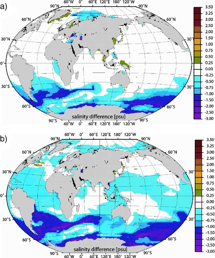
20                            D. Seidov et al. / Global and Planetary Change 49 (2005) 19–27

hemispheres. When the NA THC is weak, the northern              3. Northern versus southern meltwater sources
hemisphere (NH) is relatively cool and the southern
hemisphere (SH) is relatively warm because of weak-                The possible effects of large-scale northern fresh-
ening the northward cross-equatorial oceanic heat               water impacts in coupled atmosphere–ocean models
transport (e.g., Seidov and Maslin, 2001). When the             (AOGCMs) are a well-discussed issue (e.g., Manabe
NA THC is strong, the NH is relatively warm and the             and Stouffer, 1997; Meissner et al., 2002). In idealized
SH is relatively cool. These changes are due to the             freshwater experiments of Manabe and Stouffer, one
changes in the cross-equatorial heat transport associ-          half of the seesaw emerged when they added an
ated with the THC. This seesaw, if it exists, may be a          external source of freshwater to the NA surface (Man-
special case of a broader feature known as multiple             abe and Stouffer, 1997, 1988). In these integrations,
stability of the ocean circulation driven by freshwater         the Atlantic THC and the associated northward heat
impacts in the high latitudes (Bryan, 1986; Manabe              transport both weaken. The reduced northward heat
and Stouffer, 1988).                                            transport across the equator causes cooling of the NH
   The bi-polar seesaw metaphor has to be taken with            and warming of the SH.
caveats. Given the differences in geography in the two             Here we focus on the southern source of meltwater
hemispheres, the ocean response to northern and                 in a coupled atmosphere–ocean model. Our goal is to
southern high-latitudinal freshening/diluting may be            seek the other half of the seesaw. Can freshwater input
substantially different so that a symmetric seesaw may          in the SO cause a strengthening of the NA THC?
not exist. Therefore, the relationship of the bi-polar          Since we do not know how much or how long fresh-
seesaw, if any, to the THC response and feedback to             water should be added in the SO, our experimental
climate change may be more complicated than previ-              design is idealized.
ously discussed (e.g., Broecker, 1998; Stocker, 1998;              Some studies point out that the THC could be in
Seidov et al., 2001).                                           oscillatory regime for some sets of boundary condi-
                                                                tions during, especially related to, Dansgaard–Oesch-
                                                                ger events and 1500-period oscillation in the North
2. Freshwater and meltwater in climate models                   Atlantic (e.g., Alley et al., 2001; Bond et al., 1997;
                                                                Sakai and Peltier, 1997). However, the true seesaw
   The freshwater source for the ocean can be of four           behavior where a weakening of the SH THC causing
types—precipitation, river runoff, and sea and land ice         the NA THC to strengthen has not yet been clearly
melting. The land ice sources of freshwater to the              shown in AOGCM results.
ocean are sometimes called meltwater or glacial melt-
water and icebergs. Presumably, it is meltwater
impulses that might have caused some of the abrupt              4. Setup of experiments using coupled
climate changes on decadal and longer time scales               atmosphere–ocean model
seen in the paleo-record (e.g., Broecker et al., 1990).
   The glacial meltwater can strongly influence THC                The most complete and recent description of the
and climate by freshening the high latitude oceans.             GFDL coupled atmosphere–ocean model is given in
During major deglaciations, the ice sheets are thought          Delworth et al. (2002). In the 2001 IPCC report, this
to have supplied large amounts of meltwater and/or              model was labeled GFDL_R30 (IPCC, 2001). The
icebergs into the NA (e.g., Bond and Lotti, 1995;               coupled model consists of general circulation models
Broecker, 1998; Clark et al., 2002; Peltier and Sol-            of the atmosphere and ocean, with relatively simple
heim, 2004; Duplessy et al., 1992, 1996) and SO (e.g.,          formulations of land surface and sea ice processes (the
Duplessy et al., 1996). Many believe that both the              details of the model are discussed in Delworth et al.,
Medieval Warm Period (~ 800–1300 AD) and the                    2002; Dixon et al., 2003).
Little Ice Age (~ 1400–1900 AD) climate excursions                 The atmospheric part solves the primitive equations
are possibly related to changes in the strength of the          on a sphere using a spectral transform method. The grid
North Atlantic THC (e.g., Broecker, 2000; Broecker              uses 14 vertical levels and has an effective resolution of
and Sutherland, 2000; Cronin et al., 2003).                     roughly 3.758 longitude by 2.258 latitude. The ocean
D. Seidov et al. / Global and Planetary Change 49 (2005) 19–27                        21

component of the coupled model uses version 1.1 of the          warming the deeper layers. We also see slight weak-
Modular Ocean Model (Pacanowski et al., 1993) with              ening of the Atlantic overturning (Fig. 1a, a strength-
resolution of 1.8758 longitudes by 2.258 latitude, with         ening is expected in a bi-polar seesaw), and there is a
18 unevenly spaced levels in the vertical.                      near shutdown of the overturning cells near the Ant-
   The results of the sensitivity runs are compared             arctica coast (Fig. 1b). The hosing experiment using
with a control run (CR). The CR starts up from prior            the coupled model has not led to as large a change in
integrations of atmosphere and ocean-only models                the NA THC as in the ocean-only runs in Seidov et al.
and is driven by solar radiation with all internal              (2001). In those runs, SSS anomalies, rather than
atmospheric parameters (e.g., CO2 and other green-              anomalies of freshwater fluxes, were imposed to the
house gases concentration, vegetation, etc.), as ob-            south of Antarctic Circumpolar Current (ACC) and
served in the present-day atmosphere. Flux                      retained there. Thus, we have a weak response of the
adjustments for heat and water have been used to                Atlantic THC in the AOGCM versus a strong re-
produce realistic climate and reduce climate drift. At          sponse in the ocean-only experiments.
year 501 of the control integration, a second integra-
tion is started where a freshwater flux of 1 Sv (1
Sv = 106 m3/s) for 100 model years has been intro-              6. Southern escape
duced in the strip between 608S and the coast of
Antarctica. The word bhosingQ is used here as a                     The reason why the southern freshwater impact
shorthand way of describing the addition of the fresh-          does not lead to substantial changes of the Atlantic
water at the ocean surface. After 100 model years of            THC in the AOGCM is that the geometry of the SO
hosing, it was switched off and the integration con-            prevents the low-salinity waters from being contained
tinued for an additional 100 years. Within this period,         near the hosing (and bottom water formation) loca-
the whole system gradually recovers towards a state             tions (see Fig. 2). Although a large reduction of
that is close (though not identical) to the control             AABW formation takes place (Fig. 1b), the freshwa-
integration thus showing no significant hysteresis.             ter hosed in the SO spreads over entire SH and
                                                                eventually into the NA. As a result, instead of a
                                                                strong increase of the Atlantic THC as seen in
5. Results of experiments                                       ocean-only integrations with permanent reduction of
                                                                SSS in the SO south of the ACC (e.g., Seidov et al.,
    In the following analysis, the focus is on the THC          2001), the overturning becomes weaker in the Atlan-
and SSS changes. To save space, we present only                 tic by the end of hosing period. The spreading of the
some key variables. A longer paper is in preparation            freshwater anomaly over all the ocean basins is in
to document the full climate changes. The CR climate            sharp contrast to the northern hemisphere hosing
is very similar to that obtained using other similar            experiments (e.g., Manabe and Stouffer, 1997). In
course resolution models (see a review in IPCC,                 these experiments, the NA becomes fresher but the
2001). There is about 20 Sv of NADW formed,                     SSS over the rest of the world oceans becomes
with approximately 17 Sv exported from the Atlantic             slightly saltier.
Ocean into the SO (see Delworth et al., 2002 for more
details). The three major water masses, NADW,
AABW, and Antarctic Intermediate Water (AAIW),                  7. Ocean-only experiments with short-term
are seen in layering of salinity in the Atlantic Ocean.         freshwater hosing
    Southern hosing did not have a large influence on
the NA THC, contrary to what might have been                       Recent ocean-only experiments (e.g., Seidov et al.,
expected based on the bi-polar seesaw concept (and              2001, Seidov and Haupt, 2002) employed an idea that
ocean-only experiments with restoring boundary con-             there could be a long-term (permanent in their runs)
ditions (e.g., Seidov et al., 2001). The hosing causes          reduction of SSS in the Southern Ocean around Ant-
the deep oceanic convection to shut down around                 arctica. The nature of a freshwater source and how it
Antarctica, cooling and freshening the surface and              maintained long-term low-salinity anomaly was not
22 D. Seidov et al. / Global and Planetary Change 49 (2005) 19–27 Fig. 1. Maximum value of the annually averaged overturning stream function in the NA (a) and in the SO (b) (in Sv). It represents the strength of the THC in NA, or the rate of the NADW (a) and AABW (b) formations. Years are counted from the beginning of hosing experiments (501 years of the control run). A positive stream function value indicates a clockwise circulation looking towards the west. considered—whatever added freshwater source is, it reacts to a relatively short-term freshwater hosing, was assumed of being capable to sustain lowered similar to the one used in the coupled ocean runs surface salinity south of the ACC. described above. To address this issue, we have The ocean model was integrated to a steady state carried out an ocean-only experiment with the so- and generated a reduced AABW formation, with a called mixed boundary conditions, i.e., with specified strong spur in NADW formation. However, these SST and freshwater fluxes over the sea surface. The experiments, though fully legitimate within their freshwater fluxes that that yielded reasonably close limits, cannot give a clue of how the ocean model to observed SSS were generated using the National
D. Seidov et al. / Global and Planetary Change 49 (2005) 19–27                                          23

Fig. 2. Differences in sea surface salinity between the hosing and control runs after 25 years (a) and after 100 years (b) after beginning of the
hosing experiment.

Center for Atmospheric Research Community Cli-                                  Two snapshots of the overturning in the Atlantic
mate Model (NCAR CCM, Kiehl et al., 1998) and                               Ocean Fig. 4 at the years 2000 and 2100 confirms
kindly provided by John Dickens (Dickens, 2004).                            that there is no significant change in the overturning
The freshwater fluxes into the ocean were disturbed                         pattern, though some weakening of AABW can be
in the SO by hosing of 1 Sv of freshwater south of                          seen in Fig. 4b. However, this weakening does not
608S during 100 years at the end of 2000-year                               cause any significant NADW reduction and the THC
control run. The hosing was switched off at the                             is therefore not affected even in the Atlantic Ocean,
model year 2101 and the run then was extended to                            not speaking of the global conveyor. Thus, both
another 500 years to reveal how the ocean recovers                          ocean-only and coupled atmosphere–ocean models
from the impact.                                                            agree that intermittent short-term freshening of the
   The differences between the undisturbed SSS at                           sea surface in SO does not invoke hypothesized
2000 year and the SSS after 25, 100, 200, and 300                           increased rate of NADW formation and, therefore,
years are shown in Fig. 3. The figure shows practi-                         do not support the idea of bi-polar seesaw. However,
cally the same pattern of low-salinity signal escaping                      these experiments, ocean-only or coupled, cannot
the SO. It also indicates almost full recovery by 200                       definitively reject the idea because the nature of
years after the hosing was switched off.                                    southern freshwater impacts remains unclear. If the
24
D. Seidov et al. / Global and Planetary Change 49 (2005) 19–27
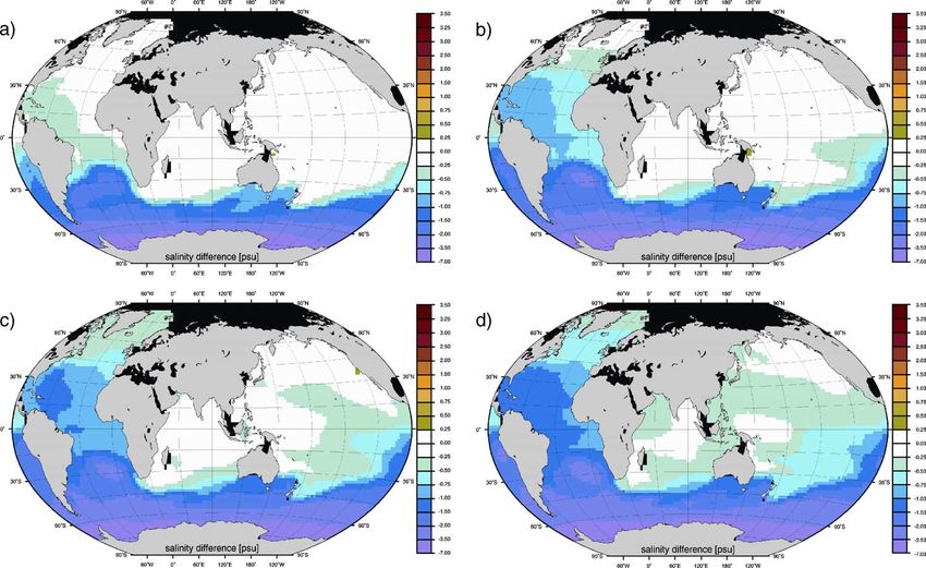
Fig. 3. Differences in sea surface salinity between the hosing and control runs in ocean-only experiments with mixed boundary conditions (see text) at model years 2025 (a), 2100 (b),
2200 (c), and 2300 (d). Freshwater hosing begins at the model year 2001 and is switched off at the model year 2101.D. Seidov et al. / Global and Planetary Change 49 (2005) 19–27 25
a) 0 -4 0
-8 8 4 8
10 4 0 0 30
40 -4 10
10 8 10
4 8 10 4 14
8
10 15 15 15 12
15 10
8
1000 20 9
15
stream function [Sv]
8
0
0
40
15 20 20 7
1
6
15
15 15
2000
depth [m]
10 5
10 10 15 4
8
8 8 8
10 3
4 4 8 10 2
3000 8 4 0 1
0 0 4
0 0
-4 -4 4 -1
4000 -2
0
-3
-4
0 -5
5000 -6
-7
-10
-20 -10 0 10 20 30 40 50 60 70 80
S Latitude [o] N
b) 0 -8 0
0 -4 10 4
8 10 84 4
815 0 84
30
104
8
15 15 10 10 14
12
20
8 10 15
15
20 10
1000 9
stream function [Sv]
20 8
15
0
15 15 15 15 7
4
2000 10 10 810 8 10 8
10 6
8 4 5
depth [m]
4 4 4 4
4 0 3
0
3000 0 0 2
0 1
-4
0
0
-1
4000 -2
-3
-4
0 0 -5
5000 -6
-7
-10
-20 -10 0 10 20 30 40 50 60 70 80
S Latitude [o] N
Fig. 4. Meridional overturning in the Atlantic Ocean in the ocean-only experiment at the model year 2000 (before freshwater hosing) and 2100
(at the end of freshwater hosing; see Fig. 3 and text). The overturning is in Sv (1 Sv = 106 m3/s).
freshening episodes are indeed strong but intermit- cause (and may also be a result) of meridional ocean
tent, the southern impacts on THC are negligible. seesaw-type oscillations.
However, if at some time in climate history they The essence of the seesaw is that reduction of
were persistent and could lower surface salinity AABW formation leads to NADW increase, whereas
around Antarctica and maintain it there, the THC a weakening of the NADW leads to an increase of
could have been altered, as some data, physical AABW production (e.g., Broecker, 1998). Although
hypothesis, and ocean modeling have suggested an ocean-only model with SSS restored towards paleo-
(e.g., Broecker, 1998; Stocker, 1998; Seidov and observations in the SO favors this line of thinking, it
Maslin, 2001). was not clear a priori, whether a coupled atmosphere–
ocean model would yield and sustain fresher surface in
the area of increased freshwater fluxes. As shown here,
8. Discussion the experiments with either the coupled model, or the
ocean-only model subjected to a short-term (about
A large concern exists about the future stability of 100-year duration) freshwater impacts in the SO do
the West Antarctic Ice Sheet (WAIS) and Greenland not substantiate containment of fresher surface in the
ice sheet as greenhouse gases increase (e.g., Gregory impact area and thus do not support the simple THC
et al., 2004; for WAIS instability see the review in seesaw paradigm. However, ocean models indicate
Oppenheimer, 1998). The line of thinking in Broecker that if a freshwater signal were of a different nature
(1998, 2000), Stocker (1998), and Weaver et al. and could have sustained a pronounced low-salinity
(2003) implied that impact of meltwater from WAIS band south of the ACC for a long time, the THC would
on AABW formation rate around Antarctica may have reacted in the predicted seesaw fashion.26 D. Seidov et al. / Global and Planetary Change 49 (2005) 19–27
Our interpretation of the radically different THC the coupled model could be due to the difference
behavior in the case of sustained and intermittent in the model setups. The ocean model was run to a
southern freshening is that this is because of funda- steady state, while the coupled model runs are
mentally different nature of southern low-salinity transient, with the time of impact limited to 100
anomalies in the two types of experiments. The years. It is unclear what the final equilibrium state
ocean-only experiments with the permanent low sur- of the coupled simulation would be like.
face salinity in the SO are based on the fact that
fresher surface water is indeed observed to the south
of the ACC in the paleo-record and it is assumed to 9. Conclusions
remain there, with the rest of the world ocean not
being freshened. Adding freshwater in the form of The bfailureQ of localized southern freshwater hos-
anomaly of freshwater fluxes rather than as a SSS ing to generate a substantial Atlantic THC change is
anomaly in either a coupled or an ocean-only model due to a fundamental difference in the nature of
allows the freshwater anomaly to spread into the rest surface freshening processes in the SO and the north-
of the world ocean. The results in the ocean-only ern NA. Because of this fundamental difference in
runs with long-term (bpermanentQ) lowering of SSS altering sea surface salinity from the two sources, the
suggest that if it had been contained, then the seesaw simple bi-polar ocean seesaw fails to develop, at least
could have emerged. Freshwater forcing, at least in in our coupled atmosphere–ocean experiments. Based
the experiments using both models presented here, on these experiments, we argue that the concept of
did not yield such containment. This is in a sharp ocean bi-polar seesaw has to be taken with some
contrast with the effect of adding an external fresh- caveats, at least.
water source to the northern NA in coupled and We also find that the boundary conditions for the
ocean-only models generating a compact and isolated ocean component play an important role in deter-
freshwater lens in the northern NA. mining the response of the model. Both types of
Thus, we have two different behaviors of ocean boundary conditions have their advantages and pro-
models in the SO, coupled and uncoupled, where blems. The freshwater boundary condition used by
the response is dependent on the boundary condi- the AOGCM has more realistic fluxes, but the SSS
tion for the oceanic component. In the NA, both anomalies may not be realistic. In the prescribed
models (coupled and uncoupled) produce a common SSS case, the anomalies are realistic, but the solu-
Atlantic THC response to freshwater impacts, re- tion may be too constrained. Moreover, the nature
gardless of whether the low surface salinity is spec- of atmosphere–ocean–cryosphere interaction that
ified (as in ocean-only models) or generated by could sustain a quasi-permanent low-salinity anom-
freshwater fluxes (e.g., Rahmstorf, 1995; Schmittner aly in the SO is not known.
and Clement, 2002). Moreover, the THC response Thus, a fundamental question remains—can SSS
to long-term low-salinity anomalies imposed over anomalies be effectively contained in the SO, instead
the sea surface or to short-term freshwater hosing of escaping from the SO, and thus whether or not an
in the same areas show similar patterns of THC ocean seesaw can develop.
reduction at the end of the hosing. This is because
in both approaches there is a well defined and
localized lens of freshened water remaining in the Acknowledgments
key areas. The attempts to simulate a confined,
localized low-salinity surface lens in the SO, as in The authors are grateful to anonymous reviewers
the northern NA, fails with both the coupled and for their very helpful and instructive comments.
the ocean models in the experiments with short-term This study was supported in part by NSF grant
freshwater impacts. #0224605. Acknowledgment is also made to the
Additionally, the differences in the results of the donors of the ACS Petroleum Research Fund
runs with SSS anomalies retained in the ocean for partial support of this research (ACS PRF
model and the anomalies in freshwater fluxes in #36812-AC8).D. Seidov et al. / Global and Planetary Change 49 (2005) 19–27 27
References Gordon, A.L., 1986. Interocean exchange of thermocline water.
Journal of Geophysical Research 91, 5037 – 5046.
Alley, R.B., Anandakrishnan, S., Jung, P., Clough, A., 2001. Sto- Gordon, A.L., Zebiak, S.E., Bryan, K., 1992. Climate variability
chastic resonance in the North Atlantic: further insights. In: and the Atlantic Ocean. Eos, Transactions-American Geophys-
Seidov, D., Haupt, B.J., Maslin, M. (Eds.), The Oceans and ical Union 79 (161), 164 – 165.
Rapid Climate Change: Past, Present, and Future. AGU, Gregory, J.M., Huybrechts, P., Raper, S.C.B., 2004. Threatened loss
Washington, DC, pp. 57 – 68. of the Greenland ice-sheet. Nature 428, 616 (8 April).
Bond, G., Lotti, R., 1995. Iceberg discharges into the North Atlantic IPCC, 2001. Climate change 2001: the scientific basis. Contribu-
on millennial time scales during the last glaciation. Science 267, tion of working group 1 to the third assessment report of the
1005 – 1010. intergovernmental panel on climate change. In: Houghton, J.T.,
Bond, G., et al., 1997. A pervasive millennial-scale cycle in North et al. (Eds.), Cambridge University Press, Cambridge, United
Atlantic Holocene and glacial climates. Science 278 (5341), Kingdom, p. 881.
1257 – 1266. Kiehl, J.T., et al., 1998. The National Center for Atmospheric
Broecker, W., 1991. The great ocean conveyor. Oceanography 1, Research Community Climate Model: CCM3. Journal of Cli-
79 – 89. mate 11 (6), 1131 – 1149.
Broecker, W.S., 1997. Thermohaline circulation, the Achilles heel Manabe, S., Stouffer, R.J., 1988. Two stable equilibria of a coupled
of our climate system: will man-made CO2 upset the current ocean–atmosphere model. Journal of Climate 1, 841 – 866.
balance? Science 278 (5343), 1582 – 1588. Manabe, S., Stouffer, R., 1997. Coupled ocean–atmosphere model
Broecker, W.S., 1998. Paleocean circulation during the last degla- response to freshwater input: comparison to Younger Dryas
ciation: a bipolar seesaw? Paleoceanography 13, 119 – 121. event. Paleoceanography 12 (2), 321 – 336.
Broecker, W.S., 2000. Was a change in thermohaline circulation Meissner, K.J., Schmittner, A., Wiebe, E.C., Weaver, A.J., 2002.
responsible for the Little Ice Age? Proceedings of the National Simulations of Heinrich Events in a coupled ocean–atmo-
Academy of Sciences 97 (4), 1339 – 1342. sphere–sea ice model. Geophysical Research Letters 29 (14),
Broecker, W.S., Sutherland, S., 2000. Distribution of carbonate ion 16-1 – 16-3.
in the deep ocean: support for a post-Little Ice Age change in Oppenheimer, M., 1998. Global warming and the stability of the
Southern ocean ventilation? Geochemistry, Geophysics, Geo- west Antarctic ice sheet. Nature 393, 325 – 332.
systems 1, 10. Pacanowski, R., Dixon, K., Rosati, A., 1993. The GFDL modular
Broecker, W.S., Bond, G., Klas, M., 1990. A salt oscillator in the ocean users guide. Geophys. Fluid Dyn. Lab.Princeton Univ.,
glacial Atlantic? 1. The concept. Paleoceanography 5 (4), Princeton, NJ.
469 – 477. Peltier, W.R., Solheim, L.P., 2004. The climate of the Earth at last
Bryan, F., 1986. High-latitude salinity effects and interhemispheric glacial maximum: statistical equilibrium state and a mode of
thermohaline circulations. Science 323, 301 – 304. internal variability. Quaternary Science Review 23, 335 – 357.
Clark, P.U., Pisias, N., Stocker, T.F., Weaver, A.J., 2002. The role of Rahmstorf, S., 1995. Multiple convection patterns and thermohaline
thermohaline circulation in abrupt climate change. Nature 415, flow in an idealized OGCM. Journal of Climate 8, 3027 – 3039.
863 – 869. Sakai, K., Peltier, W.R., 1997. Dansgaard–Oeschger oscillations in a
Cronin, T.M., Dwyer, G.S., Kamiya, T., Schwede, S., Willard, D.A., coupled atmosphere–ocean climate model. Journal of Climate
2003. Medieval warm period, Little Ice Age and 20th century 10, 949 – 970.
temperature variability from Chesapeake Bay. Global and Plan- Schmittner, A., Clement, A.C., 2002. Sensitivity of the thermoha-
etary Change 36 (1–2), 17 – 29. line circulation to tropical and high latitude freshwater forcing
Delworth, T.L., et al., 2002. Review of simulations of climate during the last glacial–interglacial cycle. Paleoceanography 17
variability and change with the GFDL R30 coupled climate (2), 7-1 – 7-12.
model. Climate Dynamics 19, 555 – 574. Seidov, D., Barron, E.J., Haupt, B.J., 2001. Meltwater and the
Dickens, J.M., 2004. Ocean–atmosphere feedback in climate simu- global ocean conveyor: northern versus southern connections.
lations using off-line modules of a coupled ocean–atmosphere Global and Planetary Change 30 (3–4), 253 – 266.
model. Master’s thesis, Pennsylvania State University, Univer- Seidov, D., Haupt, B.J., 2002. On the role of inter-basin surface
sity Park, 77 pp. salinity contrasts in global ocean circulation. Geophysical Re-
Dixon, K.W., Delworth, T.L., Knutson, T.R., Spelman, M.J., Stouffer, search Letters 29 (16), 47-1 – 47-4.
R.J., 2003. A comparison of climate change simulations produced Seidov, D., Maslin, M., 2001. Atlantic Ocean heat piracy and the bi-
by two GFDL coupled climate models. Global and Planetary polar climate sea-saw during Heinrich and Dansgaard–Oeschger
Change 37 (1–2), 81 – 102. events. Journal of Quaternary Science 16 (4), 321 – 328.
Duplessy, J.C., et al., 1992. Changes in surface salinity of the Stocker, T.F., 1998. The seesaw effect. Science 282, 61 – 62.
North Atlantic Ocean during the last deglaciation. Nature 358, Stommel, H., Arons, A.B., 1960. On the abyssal circulation of the
485 – 488. world ocean: I. Stationary planetary flow patterns on a sphere.
Duplessy, J.-C., et al., 1996. High latitude deep water sources during Deep Sea Research 6, 140 – 154.
the Last Glacial Maximum and the intensity of the global oceanic Weaver, A.J., Saenko, O.A., Clark, P.U., Mitrovica, J.X., 2003.
circulation. In: Wefer, G., Berger, W.H., Siedler, G., Webb, D. Meltwater pulse 1A from Antarctica as a trigger of the Bøl-
(Eds.), The South Atlantic. Springer, New York, pp. 445 – 460. ling–Allerød warm interval. Science 299, 1709 – 1713.You can also read