Can crude oil prices predict world tuna prices?

Songklanakarin J. Sci. Technol.
 42 (6), 1221-1226, Nov. - Dec. 2020

 Original Article

 Can crude oil prices predict world tuna prices?
 Boonmee Lee1, 2*, Mayuening Eso1, 2, Apiradee Lim1, and Don McNeil3
 1 Department of Mathematics and Computer Science, Faculty of Science and Technology,
 Prince of Songkla University, Pattani Campus, Mueang, Pattani, 94000 Thailand

 2 Centre of Excellence in Mathematics, Faculty of Science,

 Mahidol University, Ratchathewi, Bangkok, 10400 Thailand

 3Department of Statistics, Macquarie University,
 North Ryde, Northern Sydney, NSW 2109 Australia

 Received: 5 April 2019; Revised: 8 July 2019; Accepted: 20 August 2019

Abstract

 World tuna prices exhibit substantial fluctuations over time. We studied monthly tuna and preceding crude oil prices
from 1986 to 2018, using linear regression models with autoregressive and moving average (ARMA) errors. Results indicated
that a model including an increasing linear trend, the oil price 21 months earlier, and a simple ARMA(1,1) error process could
predict the monthly tuna price reasonably well for recent years, but not prior to 1999. This suggests that oil prices began to affect
tuna process only after the global financial crisis, but it takes nearly two years before a change in the oil price affects the tuna
price.

Keywords: tuna prices, crude oil prices, ARMA process, regression with autocorrelated errors, time series forecasting

1. Introduction - at around 1,260-1,270 USD/MT and will increase slightly
 for March deliveries. This seems to correspond to the cycle
 Over the past three decades, world tuna prices have of rise and fall in monthly tuna prices detected by the
exhibited substantial fluctuations, varying ±41% in monthly researchers, but variable periods of fluctuations resulted in
averages. Such fluctuations make it difficult to formulate forecasts of prices that were far behind expectations.
annual plans for tuna businesses. The previous study (Lee, In the world tuna trade, purchase contracts are
Tongkumchum, & McNeil, 2019) predicted that skipjack tuna usually agreed about two months before deliveries. To settle
prices would start falling slightly in 2018 from their peak in prices for each contract, canners and traders consider many
December 2017 of 2,308 US dollars per metric ton (USD/MT) factors, including orders for tuna products, inventories of raw
and would reach the lowest point of 1,250 USD/MT in the material in hand and on shore, number of carriers and reefers
mid 2021 before bouncing back, whereas the actual skipjack being unloaded, ongoing catchabilities, weather situations,
prices in this period had dropped much faster, to 1,300 fishing access fees, crude oil prices, and even exchange rates.
USD/MT at the end of 2018 (Thai Union Group Public Most of those factors are roughly anticipated and estimated
Company Limited, 2019). On 30 January 2019, Undercurrent while demand and supply in the tuna industry are so dynamic.
News (2019) reported that the prices were expected to hit the Therefore, the businesses have to monitor situations of world
bottom in February 2019 -- two years earlier than predictions - tuna market closely and review their business plan quarterly.
 Often, they have to revise the second half of the year plan
 when they face large discrepancies in forecasts. The need for a
*Corresponding author method of forecasting tuna prices is particularly important to
 Email address: bm_lee2001@yahoo.com the tuna industry.

1222 B. Lee et al. / Songklanakarin J. Sci. Technol. 42 (6), 1221-1226, 2020
 In exploring the information needed for negotiating
tuna prices, raw tuna suppliers usually mentioned two factors
affecting increases in offered prices. First is the bad weather
contributing to poor catchability and second is the rise of
global oil prices causing higher fishing costs. From the
literature, oil prices have been used to forecast U. S. real gross
domestic product, or GDP (Kilian & Vigfusson, 2012), and to
predict Canadian/USD exchange rates (Ferraro, Rogoff, &
Rossi, 2015). There are studies using financial data like
exchange rates to forecast commodity prices, including oil
prices (Chen, Rogoff, & Rossi, 2010). However, none of these
studies predict tuna prices or marine prices based on oil
prices. The methods used in those studies include a linear
regression, multivariate analyses using lagged independent
variables, and nonlinear models. In economic research, several
dynamic models have been developed based on regression
analysis to measure a relationship between output and inputs
for various phenomena. For example, a transfer function
model is applicable to improve forecasts of the output by
using the past observations of both the output series and the
associated input series, particularly a leading indicator (Wei,
2006). Distributed-lag models are also often used in
econometric analysis for many scenarios, in which that output
responds to specific inputs with a time lag (Gujarati, 2004).
Moreover, regression with autocorrelated errors is well-
applied in several time-series analyses (Eso, Kuning, Green,
Ueranantasun, & Chuai-Aree, 2016; Lee, McNeil, & Lim,
2017; Venables & Ripley, 2002) because it provides the
ability to model both the signal and the noise at the same time
and gives more accurate results. With those valid methods, we
then aim to investigate how oil prices, influencing major costs
in tuna fishing operations, influence tuna prices and seek a
method that enables global oil prices to predict world tuna
prices over time.

2. Materials and Methods
 The two datasets used in this study are commodity Figure 1. (a) Relation between the logarithm of standard deviation
prices data from 1986 to 2018. The first dataset is the monthly and the logarithm of mean of annual oil price. (b) A normal
skipjack tuna price in US dollars (USD) per metric ton (MT) quantile-quantile plot of studentized residuals of the linear
collected from three sources: Atuna (2017), Food and model after fitting log-transformed oil prices.
Agriculture Organization of the United Nations (FAO, 2014),
and Thai Union Group Public Company Limited (2019). The As time-series prediction is the primary interest in
second dataset is the monthly crude oil price of West Texas this study, we followed the regression with autocorrelated
Intermediate in US dollars per barrel provided by the U.S. errors method in section 14.5 (Venables & Ripley, 2002).
Energy Information Administration (2019). This method can be simply implemented by using the arima()
 The monthly tuna prices required a logarithmic function in R program. The function enables us to easily add
transformation to stabilize the variance of time series, and an external regression vector into the model in order to
needed a seasonal adjustment before statistical modeling (Lee analyze the signal (regressions with time and independent
et al., 2019). The monthly oil prices also needed log- variables) and the noise (autocorrelation) at the same time (R
transformation, as illustrated in Figure 1, in which (a) the plot Core Team, 2017). With this method capability, time was also
of standard deviations against means of annual oil prices after included in the regressions for analyzing a direction of trend.
logarithmic transform shows a linear relationship, and (b) the For the noise analysis, both autocorrelation function (ACF)
studentized residuals from the log-linear model are normally and partial autocorrelation function (PACF) of the model
distributed in the normal quantile-quantile plot. Thus, residuals were iteratively plotted until they successfully
seasonally adjusted log-transformed tuna prices and log- described white noise conditions in order to determine
transformed oil prices were used to investigate the relationship appropriate orders of autoregressive AR(p), moving average
between tuna price fluctuations and oil price movements, and MA(q) or mixed autoregressive moving average ARMA(p,q)
to develop a forecasting model for world tuna prices. All processes (Box & Jenkins, 1970). Regarding the model
statistical methods were carried out using the R program (R properties in section 14.2 (Venables & Ripley, 2002), an
Core Team, 2017). MA(q) process always defines a stationary time series but the
 AR(p) and ARMA(p,q) processes can be stationary or non-

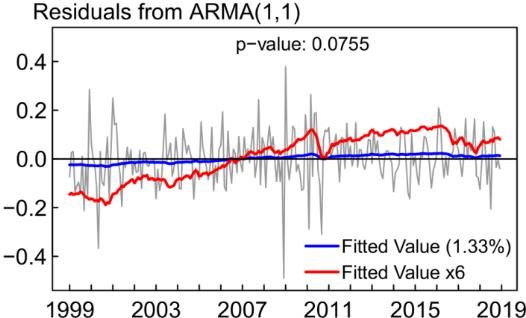
B. Lee et al. / Songklanakarin J. Sci. Technol. 42 (6), 1221-1226, 2020 1223
stationary. Being aware that model building for price data is
linked with economics and business in this particular case, a
nonstationary time series is possible. To ensure the model
errors are properly handled, fitted values from separately
fitting a simple linear regression to the trend component and
to the noise component of the proposed model were examined
as well.
 In this application, we focus on predicting monthly
tuna prices at least one year ahead by considering tuna and oil
prices at lags of 12 to 24 months together with time as an
initial explanatory variable in the regression. To seek the best
combination of determinants that provide predictive power for
tuna prices, the analyses involved fitting the regression with Figure 2. Monthly world tuna prices and global oil prices in log-
errors based on ARMA(p,q) process to the data and backward scale, 1986-2018.
eliminating those insignificant lagged values with the highest
or greater than 0.05 p-values, one-by-one, until there remained
only significant lagged terms. Thus, the forecasts of world
tuna prices were derived from modeling both the trend and the
errors with a combination of significant lagged dependent and
independent variables. To estimate the MA(q) parameters for
the forecasts, bootstrap resampling (Efron & Tibshirani, 1998)
was also used.

3. Results
 The graph in Figure 2 illustrates the seasonally
adjusted tuna prices and oil prices from 1986 to 2018 in log-
scale. It shows the oil prices dropping significantly during the
economic crisis of 1997-1998 before starting to greatly
increase in 1999. Tuna industry experienced a collapse of the
skipjack prices during 1999-2000 because of oversupply,
before the prices were stabilized by reducing fishing efforts in
the following year (Hamilton et al., 2011). Graphically, these
commodity prices had some similarities in their rises and falls.
The statistical results of p-values < 0.001 from fitting an
additive model to the entire 34-year series of seasonally-
adjusted log-transformed tuna prices with similarly trans-
formed oil prices as the independent variables indicate that
there is a dynamic relationship between oil prices and world Figure 3. Data autocorrelation of tuna prices (left panel) with
tuna prices, but its regression predictions can explain future coefficients of statistically significant autoregressive and
movements in tuna prices for only 42%. moving average parameters; Residual autocorrelation of
 Looking at the price variations over the three the regression with ARMA(1,1) errors model (right panel).
decades in Figure 2, the patterns suggest two periods. The first
period from 1986 to 1998 shows no trend and no relation past value at lag 1, when fitting the model simultaneously.
between oil prices and tuna prices, and statistical testing After the iterative process of regressions with ARMA(1,1)
confirmed this by accepting the null hypothesis with p-value errors and backward eliminations, only two predictors - time
0.97. However, the second period from 1999 to 2018 demon- and oil price at lag 21 remained significant, with p-values
strates an increasing trend in both prices, and validity test smaller than 0.05, as shown in Table 1. The coefficients in this
gave p-values < 0.0001, coefficient 0.37, and a higher r- final model are positive. The coefficient of time, 0.0037 is
squared of 55%. Obviously, global oil prices do affect world almost negligible but gives a slight upward trend to world tuna
tuna prices. The average oil prices of this second period prices over time. The coefficient 0.1454 indicates that crude
climbed up three-fold, to 60 USD/barrel from 19 USD/barrel oil prices from 21 months ago are considerably associated
in the first period. Average tuna prices also increased, but by a with world tuna prices.
smaller percentage to 1,208 USD/MT from 886 USD/MT. When fitting the linear regression model to tuna
Therefore, only monthly prices from January 1999 to prices with the two suggested predictors (time and oil price at
December 2018 were used for the model building. lag 21), the fitted values to tuna prices had a 68.34%
 From data autocorrelation diagnoses, the ARMA goodness-of-fit, as illustrated in Figure 4 (left panel). When
(1,1) process was found most appropriate to constitute we applied the same linear regression with the two
successive white noises with AR1 and MA1 coefficients of determinants to the residual series, which remained from
0.946 and 0.307 respectively, as shown in Figure 3. This fitting the regression with ARMA(1,1) model, predicted
implies that the monthly price of tuna greatly depends on the values of the noise in Figure 4 (right panel) exhibited an

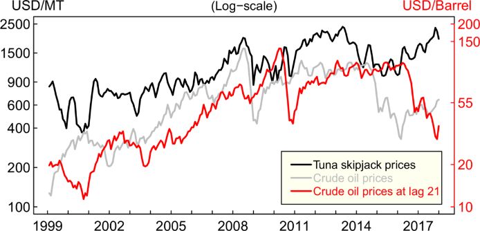
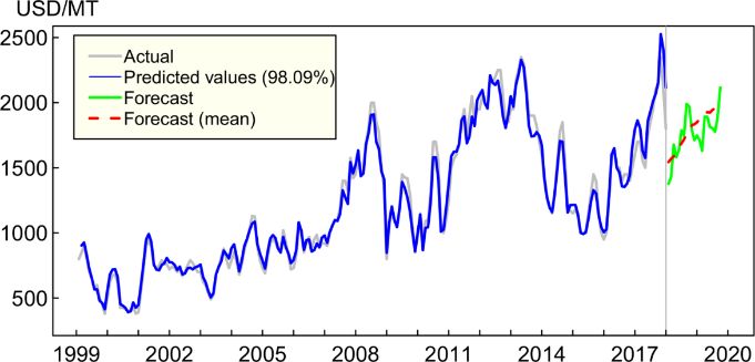
1224 B. Lee et al. / Songklanakarin J. Sci. Technol. 42 (6), 1221-1226, 2020
Table 1. The coefficients in the regression with two combined
 predictors and ARMA(1,1) error model.

 Parameter Coefficient Std. error z-value p-value

 ar1 0.8393 0.0390 21.536 < 0.001
 ma1 0.3503 0.0655 5.349 < 0.001
 (Intercept) 5.4377 0.2682 20.273 < 0.001
 Time 0.0037 0.0009 4.192 < 0.001
 Oil prices at 0.1454 0.0730 1.991 0.047
 lag 21

 Figure 5. Monthly world tuna prices and 21-lagged oil prices in log-
 scale, 1999-2018.

 Figure 6. Predicted values and forecasts for world tuna prices.

 noise was repeated 1,000 times in order to get the average
 values for final forecasts of each month, which were labeled
 as “Forecast (mean)”, the red dashed line in the graph, while
 the green line, “Forecast” was derived from a one-time
 random sampling.
 By comparing to a previous study (Lee et al., 2019)
Figure 4. Predicted values from the linear regression model with the as shown in Table 2, combing oil price as predictor in this
 two combined predictors: modeling the signal (left panel) study improves the monthly forecasts of tuna prices, esti-
 and modeling the noise from the regression with mating lower average prices in year 2019 at 1,701 USD/MT.
 ARMA(1,1) errors model (right panel). The model predicts an upward trend in tuna prices with
 quarterly prices at 1564, 1655, 1752 and 1833 USD/MT, and
increasing trend of variations, exactly as the ones of the signal will slightly rise to peak at 1,954 USD/MT in July 2020
(left panel) with p-value greater than 0.05, indicating that the before dropping, corresponding to the fall of global oil prices
proposed model completely handles the noise and fluctuations from 70 to 57 USD/barrel 21 months prior to that.
of world tuna prices with likely random noise perturbations.
The results show that it takes 21 months before a change in 4. Discussion and Conclusions
the oil price affects the tuna price, and such relationship is re-
illustrated in Figure 5. This study discovered that global oil prices can be
 As depicted in Figure 6, the forecasts were used to predict world tuna prices. We investigated monthly
calculated using the following formula: data from 1986 to 2018 and found a dynamic relationship
 between tuna price fluctuations and oil price movements in
 (1 + 0.3503 ) recent years, but not prior to 1999. Such relationship appears
 = 5.4377 + 0.0037 + 0.1454 −21 + 
 (1 − 0.8393 ) to be robust and to hold when we combine lagged tuna and oil
 prices in the regressions. By following the first principle of
In the model, represents the seasonally adjusted log- statistics, the regression with autocorrelated errors not only
transformed tuna price for period t, starting from January provides an ability to model the signal and the noise at the
1999, −21 is log-transformed oil price, B is the backshift same time but also importantly enables global oil prices to
operator for order of ARMA process, and is a white noise predict world tuna prices at least one year ahead.
series with zero mean and constant variance. The predicted The fluctuations in tuna prices have had similar
values can explain past observations almost perfectly with random noise occurring over time, illustrating dynamic cycles
adjusted r-squared 98%. In order to calculate the forecasts of in the tuna supply-chain from farm to folk, typically short-
this model, we had to generate white noise randomly term supply imbalances. To avoid a misleading impression of
sampled from the residuals of the model, and then added to economic cycles accumulated in the data, determining
the predicted trend. This bootstrap resampling for random appropriate orders for an AR or ARMA model in this study is

B. Lee et al. / Songklanakarin J. Sci. Technol. 42 (6), 1221-1226, 2020 1225
 Table 2. Comparative forecasts for world tuna prices.

 2018 Forecasts for 2019
 Actual
 price Linear Combining
 Month Linear Combining
 in spline model* oil prices as predictors spline oil prices as
 2018
 model* predictors
 Forecasts %Err Fitted value %Err

 1 1550 2160 39.4 1708 10.2 2117 1542
 2 1480 2191 48.0 1584 7.0 2078 1567
 3 1700 2216 30.4 1788 5.2 2037 1583
 4 1800 2236 24.2 1889 4.9 1993 1624
 5 1600 2250 40.6 1690 5.6 1948 1657
 6 1600 2256 41.0 1639 2.4 1902 1685
 7 1300 2254 73.4 1319 1.5 1855 1715
 8 1450 2246 54.9 1393 -4.0 1808 1759
 9 1650 2231 35.2 1614 -2.2 1762 1781
 10 1525 2210 44.9 1567 2.7 1716 1822
 11 1400 2183 55.9 1517 8.4 1672 1831
 12 1300 2125 63.5 1433 10.2 1629 1846

 Average
 1530 2213 44.7 1595 4.3 1876 1701
 in year

 MAPE 45.9 5.4

 Notes: *Results from a previous study (Lee et al., 2019)

very crucial. Looking at the ACF and PACF plots alone is fishing operation, from the start till tunas are transshipped and
inadequate because significant correlated errors were totally unloaded at the destination port. This study statistically found
eliminated with about the same results in the plots when trying that it takes nearly two years, a long lead-time, for the landing
different orders in the iterative process. At the first try, it prices of tuna to reflect acquisition costs of crude oil a refiner
obviously suggested AR(2) when we diagnosed autocorrela- paid for. This draws attention to potential further studies on
tions of either the signal (tuna prices series) or the noise other dynamic models, such as transfer function model and
(residuals series from the linear regression). The AR(2) distributed-lag, in order to compare similarities and dif-
process constitutes white noise conditions and coefficients of ferences in results.
parameters AR1 and AR2 are 1.214 and -0.257 respectively.
However, when regressing tuna prices with past values of both Acknowledgements
tuna and oil prices based on AR(2) process, none of the lagged
variables is significant. This does not meet our ultimate goal This study was supported by a Ph.D. Overseas
to predict tuna prices with oil prices. Then, we tried the mixed Thesis Research from Prince of Songkla University, Thailand
ARMA(2,1) process whose parameter estimates also success- and partially funded by the Centre of Excellence in
fully described white noise conditions, but it was found that Mathematics, the Commission on Higher Education, Thailand.
the estimated parameter of AR2 is much smaller than its We wish to acknowledge Professor Sung K. Ahn and
standard error. Finally, we found that the mixed ARMA(1,1) Department of Finance & Management Science, Carson
is the most appropriate model and the model suggested only College of Business, WSU for supporting data sources used in
two valid predictors – time and oil price at lag 21. this study, and to thank two anonymous reviewers for
 The model gives global oil prices a predictive power comments and suggestions that improved our article
for 12-month-ahead forecasts of world tuna prices, being substantially.
useful for tuna industry to prepare annual business plans. It
predicts an upward trend in monthly tuna prices with an References
average of 1,701 USD/MT for year 2019, and the trend having
an opposite direction to the forecasts derived from the Atuna. (2017, December 21). Frozen Skipjack whole round
previous linear spline model (Lee et al., 2019). This is 1.8kg up CFR Bangkok. Retrieved from http://
because the duration of a future cycle is shorter than the www.atuna.com/index.php/en/tuna-prices/skipjack
historical ones, and prices in 2018 had dropped four times -cfr-bangkok
faster than the prediction from the linear spline model, falling Box, G. E. P., & Jenkins, G. M. (1970). Time series analysis:
about 1,000 USD/MT within a year. Considering the actual Forecasting and control. San Francisco, CA:
prices at the end of 2018 (1,300 USD/MT), forecasts in this Holden-Day.
study may be a little aggressive because they mainly have Chen, Y., Rogoff, K. S., & Rossi, B. (2010). Can Exchange
been influenced by increasing prices of crude oil, 21 months Rates Forecast Commodity Prices? The Quarterly
ago. There is a lead-time for crude oil to be refined into Journal of Economics, 125(3), 1145–1194. doi:
gasoline and delivered to retail gas stations in each fishing 10.1162/qjec.2010.125.3.1145
country. Furthermore, it takes a few months for the tuna

1226 B. Lee et al. / Songklanakarin J. Sci. Technol. 42 (6), 1221-1226, 2020
Efron, B., & Tibshirani, R. J. (1998). An introduction to the Statistics Conference 2017: Enhancing Statistics,
 bootstrap. New York, NY: CRC Press LLC. Prospering Human Life. Voorburg, Netherland.
Eso, M., Kuning, M., Green, H., Ueranantasun, A., & Chuai- Lee, B., Tongkumchum, P., & McNeil, D. (2019). Forecasting
 Aree, S. (2016). The Southern Oscillation Index as a monthly world tuna prices with a plausible
 Random Walk. Walailak Journal of Science and approach. Songklanakarin Journal of Science and
 Technology, 13, 317-327. Technology, (In press).
Food and Agriculture Organization of the United Nations. R Core Team. (2017). R: A language and environment for
 (2014). Globefish Commodity Update May 2014: statistical computing. R foundation for statistical
 Tuna. Retrieved from http://www.fao.org/in-action/ computing, Vienna, Austria. Retrieved from https://
 globefish/publications/details- www.R-project.org/
 publication/en/c/356793/ Thai Union Group Public Company Limited. (2019, February
Ferraro, D., Rogoff, K. S., & Rossi, B. (2015). Can oil prices 16). Monthly frozen (whole) skipjack tuna raw
 forecast exchange rates? An empirical analysis of material prices (Bangkok landings, WPO). Re-
 the relationship between commodity prices and trieved from http://investor.thaiunion.com/raw_
 exchange rates. Journal of International Money and material.html
 Finance, 54(June), 116-141. doi:10.1016/j.jimonfin. U. S. Energy Information Administration. (2019, February
 2015.03.001 16). Crude oil prices: West Texas Intermediate
Gujarati, D. N. (2004). Basic econometrics (4th ed.). New (WTI) - Cushing, Oklahoma [DCOILWTICO]. Re-
 York, NY: The McGraw−Hill Companies. trieved from https://fred.stlouisfed.org/series/DCOI
Hamilton, A., Lewis, A., McCoy, M. M., Havice, E., & LWTICO
 Campling, L. (2011) Market and industry dynamics Undercurrent News. (2019, January 30). Skipjack tuna prices
 in the global tuna supply chain. Pacific Islands likely at bottom in Bangkok, Manta. Retrieved from
 Forum Fisheries Agency, Honiara, Solomon Islands. https://www.undercurrentnews.com/2019/01/30/skip
Kilian, L., & Vigfusson, R. J. (2012). Do oil prices help jack-tuna-prices-likely-at-bottom-in-bangkok-man
 forecast U.S. real GDP? The role of nonlinearities ta/
 and asymmetries. Journal of Business and Economic Venables, W. N., & Ripley, B. D. (2002). Modern applied sta-
 Statistics, 31(1), 78-93. doi:10.1080/07350015.20 tistics with S (4th ed.). London, England: Springer.
 12.740436 Wei, W. W. S. (2006). Time series analysis: Univariate and
Lee, B., McNiel, D., & Lim, A. (2017). Spline interpolation multivariate methods (2nd ed.). Boston, MA: Pearson
 for forecasting world tuna catches. Proceeding of Education.
 The International Statistical Institute Regional