Learning Depth from Single Monocular Images
←
→
Page content transcription
If your browser does not render page correctly, please read the page content below
Learning Depth from Single Monocular Images

                 Ashutosh Saxena, Sung H. Chung, and Andrew Y. Ng
                            Computer Science Department
                                Stanford University
                                Stanford, CA 94305
                            asaxena@stanford.edu,
                     {codedeft,ang}@cs.stanford.edu

                                        Abstract
         We consider the task of depth estimation from a single monocular im-
         age. We take a supervised learning approach to this problem, in which
         we begin by collecting a training set of monocular images (of unstruc-
         tured outdoor environments which include forests, trees, buildings, etc.)
         and their corresponding ground-truth depthmaps. Then, we apply su-
         pervised learning to predict the depthmap as a function of the image.
         Depth estimation is a challenging problem, since local features alone are
         insufficient to estimate depth at a point, and one needs to consider the
         global context of the image. Our model uses a discriminatively-trained
         Markov Random Field (MRF) that incorporates multiscale local- and
         global-image features, and models both depths at individual points as
         well as the relation between depths at different points. We show that,
         even on unstructured scenes, our algorithm is frequently able to recover
         fairly accurate depthmaps.

1   Introduction
Recovering 3-D depth from images is a basic problem in computer vision, and has im-
portant applications in robotics, scene understanding and 3-D reconstruction. Most work
on visual 3-D reconstruction has focused on binocular vision (stereopsis) [1] and on other
algorithms that require multiple images, such as structure from motion [2] and depth from
defocus [3]. Depth estimation from a single monocular image is a difficult task, and re-
quires that we take into account the global structure of the image, as well as use prior
knowledge about the scene. In this paper, we apply supervised learning to the problem
of estimating depth from single monocular images of unstructured outdoor environments,
ones that contain forests, trees, buildings, people, buses, bushes, etc.
In related work, Michels, Saxena & Ng [4] used supervised learning to estimate 1-D dis-
tances to obstacles, for the application of autonomously driving a remote control car. Nagai
et al. [5] performed surface reconstruction from single images for known, fixed, objects
such as hands and faces. Gini & Marchi [6] used single-camera vision to drive an in-
door robot, but relied heavily on known ground colors and textures. Shape from shading
[7] offers another method for monocular depth reconstruction, but is difficult to apply to
scenes that do not have fairly uniform color and texture. In work done independently of
ours, Hoiem, Efros and Herbert (personal communication) also considered monocular 3-D
reconstruction, but focused on generating 3-D graphical images rather than accurate met-
ric depthmaps. In this paper, we address the task of learning full depthmaps from single
images of unconstrained environments.
Markov Random Fields (MRFs) and their variants are a workhorse of machine learning,
and have been successfully applied to numerous problems in which local features were in-
sufficient and more contextual information had to be used. Examples include text segmen-
tation [8], object classification [9], and image labeling [10]. To model spatial dependencies
in images, Kumar and Hebert’s Discriminative Random Fields algorithm [11] uses logistic
regression to identify man-made structures in natural images. Because MRF learning is
intractable in general, most of these model are trained using pseudo-likelihood.
Our approach is based on capturing depths and relationships between depths using an MRF.
We began by using a 3-D distance scanner to collect training data, which comprised a
large set of images and their corresponding ground-truth depthmaps. Using this training
set, the MRF is discriminatively trained to predict depth; thus, rather than modeling the
joint distribution of image features and depths, we model only the posterior distribution
of the depths given the image features. Our basic model uses L2 (Gaussian) terms in
the MRF interaction potentials, and captures depths and interactions between depths at
multiple spatial scales. We also present a second model that uses L1 (Laplacian) interaction
potentials. Learning in this model is approximate, but exact MAP posterior inference is
tractable (similar to Gaussian MRFs) via linear programming, and it gives significantly
better depthmaps than the simple Gaussian model.
2 Monocular Cues
Humans appear to be extremely good at judging depth from single monocular images. [12]
This is done using monocular cues such as texture variations, texture gradients, occlusion,
known object sizes, haze, defocus, etc. [4, 13, 14] For example, many objects’ texture will
look different at different distances from the viewer. Texture gradients, which capture the
distribution of the direction of edges, also help to indicate depth.1 Haze is another depth
cue, and is caused by atmospheric light scattering.
Most of these monocular cues are “contextual information,” in the sense that they are global
properties of an image and cannot be inferred from small image patches. For example, oc-
clusion cannot be determined if we look at just a small portion of an occluded object.
Although local information such as the texture and color of a patch can give some informa-
tion about its depth, this is usually insufficient to accurately determine its absolute depth.
For another example, if we take a patch of a clear blue sky, it is difficult to tell if this patch
is infinitely far away (sky), or if it is part of a blue object. Due to ambiguities like these,
one needs to look at the overall organization of the image to determine depths.
3 Feature Vector
In our approach, we divide the image into small patches, and estimate a single depth value
for each patch. We use two types of features: absolute depth features—used to estimate the
absolute depth at a particular patch—and relative features, which we use to estimate relative
depths (magnitude of the difference in depth between two patches). We chose features that
capture three types of local cues: texture variations, texture gradients, and haze.
Texture information is mostly contained within the image intensity channel,2 so we apply
Laws’ masks [15, 4] to this channel to compute the texture energy (Fig. 1). Haze is reflected
in the low frequency information in the color channels, and we capture this by applying a
local averaging filter (the first Laws mask) to the color channels. Lastly, to compute an
1
For example, a tiled floor with parallel lines will appear to have tilted lines in an image. The dis-
tant patches will have larger variations in the line orientations, and nearby patches will have smaller
variations in line orientations. Similarly, a grass field when viewed at different distances will have
different texture gradient distributions.
2
We represent each image in YCbCr color space, where Y is the intensity channel, and Cb and Cr
are the color channels.Figure 1: The convolutional filters used for texture energies and gradients. The first nine are
3x3 Laws’ masks. The last six are the oriented edge detectors spaced at 300 intervals. The
nine Law’s masks are used to perform local averaging, edge detection and spot detection.
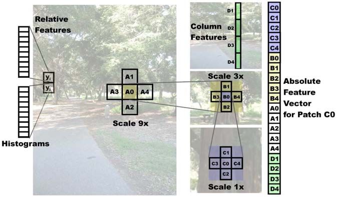
Figure 2: The absolute depth feature vector for a patch, which includes features from its
immediate neighbors and its more distant neighbors (at larger scales). The relative depth
features for each patch use histograms of the filter outputs.
estimate of texture gradient that is robust to noise, we convolve the intensity channel with
six oriented edge filters (shown in Fig. 1).
3.1 Features for absolute depth
Given some patch i in the image I(x, y), we compute summary statistics for it as follows.
We use the output of each of the 17 (9 Laws’ masks, P2 color channels and 6 texture gra-
dients) filters Fn (x, y), n = 1, ..., 17 as: Ei (n) = (x,y)∈patch(i) |I(x, y) ∗ Fn (x, y)|k ,
where k = {1, 2} give the sum absolute energy and sum squared energy respectively. This
gives us an initial feature vector of dimension 34.
To estimate the absolute depth at a patch, local image features centered on the patch are
insufficient, and one has to use more global properties of the image. We attempt to capture
this information by using image features extracted at multiple scales (image resolutions).
(See Fig. 2.) Objects at different depths exhibit very different behaviors at different resolu-
tions, and using multiscale features allows us to capture these variations [16]. 3 In addition
to capturing more global information, computing features at multiple spatial scales also
help accounts for different relative sizes of objects. A closer object appears larger in the
image, and hence will be captured in the larger scale features. The same object when far
away will be small and hence be captured in the small scale features. Such features may be
strong indicators of depth.
To capture additional global features (e.g. occlusion relationships), the features used to
predict the depth of a particular patch are computed from that patch as well as the four
neighboring patches. This is repeated at each of the three scales, so that the feature vector
3
For example, blue sky may appear similar at different scales; but textured grass would not.at a patch includes features of its immediate neighbors, and its far neighbors (at a larger
scale), and its very far neighbors (at the largest scale), as shown in Fig. 2. Lastly, many
structures (such as trees and buildings) found in outdoor scenes show vertical structure, in
the sense that they are vertically connected to themselves (things cannot hang in empty air).
Thus, we also add to the features of a patch additional summary features of the column it
lies in.
For each patch, after including features from itself and its 4 neighbors at 3 scales, and
summary features for its 4 column patches, our vector of features for estimating depth at a
particular patch is 19 ∗ 34 = 646 dimensional.
3.2 Features for relative depth
We use a different feature vector to learn the dependencies between two neighboring
patches. Specifically, we compute a histogram (with 10 bins) of each of the 17 filter outputs
|I(x, y) ∗ Fn (x, y)|, giving us a total of 170 features yi for each patch i. These features
are used to estimate how the depths at two different locations are related. We believe that
learning these estimates requires less global information than predicting absolute depth, 4
but more detail from the individual patches. Hence, we use as our relative depth features the
differences between the histograms computed from two neighboring patches y ij = yi − yj .
4 The Probabilistic Model
The depth of a particular patch depends on the features of the patch, but is also related to
the depths of other parts of the image. For example, the depths of two adjacent patches
lying in the same building will be highly correlated. We will use an MRF to model the
relation between the depth of a patch and the depths of its neighboring patches. In addition
to the interactions with the immediately neighboring patches, there are sometimes also
strong interactions between the depths of patches which are not immediate neighbors. For
example, consider the depths of patches that lie on a large building. All of these patches
will be at similar depths, even if there are small discontinuities (such as a window on the
wall of a building). However, when viewed at the smallest scale, some adjacent patches
are difficult to recognize as parts of the same object. Thus, we will also model interactions
between depths at multiple spatial scales.
Our first model will be a jointly Gaussian MRF. To capture the multiscale depth relations,
define di (s) as follows. For each of three scales s = 1, 2, 3, define di (s + 1) =
let us P
(1/5) j∈Ns (i)∪{i} dj (s). Here, Ns (i) are the 4 neighbors of patch i at scale s. I.e., the
depth at a higher scale is constrained to be the average of the depths at lower scales. Our
model over depths is as follows:
M T 2 3 X M X (di (s) − dj (s))2
1 X (d i (1) − x i θ r ) X
P (d|X; θ, σ) = exp − 2 − 2
Z i=1
2σ 1r s=1 i=1
2σ 2rs
j∈Ns (i)
(1)
Here, M is the total number of patches in the image (at the lowest scale); xi is the absolute
depth feature vector for patch i; and θ and σ are parameters of the model. In detail, we
use different parameters (θr , σ1r , σ2r ) for each row in the image, because the images we
consider are taken from a horizontally mounted camera, and thus different rows of the
image have different statistical properties.5 Z is the normalization constant for the model.
4
For example, given two adjacent patches of a distinctive, unique, color and texture, we may be
able to safely conclude that they are part of the same object, and thus that their depths are close, even
without more global features.
5
For example, a blue patch might represent sky if it is in upper part of image, and might be more
likely to be water if in the lower part of the image.We estimate the parameters θr in Eq. 1 by maximizing the conditional likelihood
p(d|X; θr ) of the training data. Since the model is a multivariate Gaussian, the maximum
likelihood estimate of parameters θr is obtained by solving a linear least squares problem.
The first term in the exponent above models depth as a function of multiscale features of a
single patch i. The second term in the exponent places a soft “constraint” on the depths to
2
be smooth. If the variance term σ2rs is a fixed constant, the effect of this term is that it tends
to smooth depth estimates across nearby patches. However, in practice the dependencies
between patches are not the same everywhere, and our expected value for (d i − dj )2 may
depend on the features of the local patches.
2
Therefore, to improve accuracy we extend the model to capture the “variance” term σ 2rs
in the denominator of the second term as a linear function of the patches i and j’s relative
2
depth features yijs (discussed in Section 3.2). We use σ2rs = uTrs |yijs |. This helps deter-
mine which neighboring patches are likely to have similar depths. E.g., the “smoothing”
effect is much stronger if neighboring patches are similar. This idea is applied at multiple
2
scales, so that we learn different σ2rs for the different scales s (and rows r of the image).
2
The parameters urs are chosen to fit σ2rs to the expected value of (di (s) − dj (s))2 , with a
2
constraint that urs ≥ 0 (to keep the estimated σ2rs non-negative).
2 2
Similar to our discussion on σ2rs , we also learn the variance parameter σ1r = vrT xi as a
2
linear function of the features. The parameters vr are chosen to fit σ1r to the expected value
of (di (r) − θrT xi )2 , subject to vr ≥ 0.6 This σ1r
2
term gives a measure of the uncertainty
in the first term, and depends on the features. This is motivated by the observation that in
some cases, depth cannot be reliably estimated from the local features. In this case, one
has to rely more on neighboring patches’ depths to infer a patch’s depth (as modeled by the
second term in the exponent).
After learning the parameters, given a new test-set image we can find the MAP estimate of
the depths by maximizing Eq. 1 in terms of d. Since Eq. 1 is Gaussian, log P (d|X; θ, σ)
is quadratic in d, and thus its maximum is easily found in closed form (taking at most 2-3
seconds per image, including feature computation time).
4.1 Laplacian model
We now present a second model that uses Laplacians instead of Gaussians to model the
posterior distribution of the depths. Our motivation for doing so is three-fold. First, a
histogram of the relative depths (di − dj ) empirically appears Laplacian, which strongly
suggests that it is better modeled as one. Second, the Laplacian distribution has heavier
tails, and is therefore more robust to outliers in the image features and error in the training-
set depthmaps (collected with a laser scanner; see Section 5.1). Third, the Gaussian model
was generally unable to give depthmaps with sharp edges; in contrast, Laplacians tend to
model sharp transitions/outliers better. Our model is as follows:
M T 3 X M
1 X |d i (1) − x θ
i r | X X |d i (s) − d j (s)|
P (d|X; θ, λ) = exp − − (2)
Z i=1
λ 1r s=1 i=1
λ 2rs
j∈Ns (i)
Here, the parameters are the same as Eq. 1, except for the variance terms. Here, λ 1r and
λ2rs are the Laplacian spread parameters. Maximum-likelihood parameter estimation for
the Laplacian model is not tractable (since the partition function depends on θ r ). But by
analogy to the Gaussian case, we approximate this by solving a linear system of equations
Xr θr ≈ dr to minimize L1 (instead of L2 ) error. Here Xr is the matrix of absolute-depth
features. Following the Gaussian model, we also learn the Laplacian spread parameters
in the denominator in the same way, except that the instead of estimating the expected
value of (di − dj )2 , we estimate the expected value of |di − dj |. Even though maximum
6 2
The absolute depth features xir are non-negative; thus, the estimated σ1r is also non-negative.likelihood parameter estimation for θr is intractable in the Laplacian model, given a new test-set image, MAP inference for the depths d is tractable. Specifically, P (d|X; θ, λ) is easily maximized in terms of d using linear programming. Remark. We can also extend these models to combine Gaussian and Laplacian terms in the exponent, for example by using a L2 norm term for absolute depth, and a L1 norm term for the interaction terms. MAP inference remains tractable in this setting, and can be solved using convex optimization as a QP (quadratic program). 5 Experiments 5.1 Data collection We used a 3-D laser scanner to collect images and their corresponding depthmaps. The scanner uses a SICK 1-D laser range finder mounted on a motor to get 2D scans. We col- lected a total of 425 image+depthmap pairs, with an image resolution of 1704x2272 and a depthmap resolution of 86x107. In the experimental results reported here, 75% of the im- ages/depthmaps were used for training, and the remaining 25% for hold-out testing. Due to noise in the motor system, the depthmaps were not perfectly aligned with the images, and had an alignment error of about 2 depth patches. Also, the depthmaps had a maximum range of 81m (the maximum range of the laser scanner), and had minor additional errors due to reflections and missing laser scans. Prior to running our learning algorithms, we transformed all the depths to a log scale so as to emphasize multiplicative rather than addi- tive errors in training. In our earlier experiments (not reported here), learning using linear depth values directly gave poor results. 5.2 Results We tested our model on real-world test-set images of forests (containing trees, bushes, etc.), campus areas (buildings, people, and trees), and indoor places (such as corridors). The algorithm was trained on a training set comprising images from all of these environments. Table 1 shows the test-set results when using different feature combinations. We see that using multiscale and column features significantly improves the algorithm’s performance. Including the interaction terms further improved its performance, and the Laplacian model performs better than the Gaussian one. Empirically, we also observed that the Laplacian model does indeed give depthmaps with significantly sharper boundaries (as in our discus- sion in Section 4.1; also see Fig. 3). Table 1 shows the errors obtained by our algorithm on a variety of forest, campus, and indoor images. The results on the test set show that the algorithm estimates the depthmaps with a average error of 0.132 orders of magnitude. It works well even in the varied set of environments as shown in Fig. 3 (last column). It also appears to be very robust towards variations caused by shadows. Informally, our algorithm appears to predict the relative depths of objects quite well (i.e., their relative distances to the camera), but seems to make more errors in absolute depths. Some of the errors can be attributed to errors or limitations of the training set. For example, the training set images and depthmaps are slightly misaligned, and therefore the edges in the learned depthmap are not very sharp. Further, the maximum value of the depths in the training set is 81m; therefore, far-away objects are all mapped to the one distance of 81m. Our algorithm appears to incur the largest errors on images which contain very irregular trees, in which most of the 3-D structure in the image is dominated by the shapes of the leaves and branches. However, arguably even human-level performance would be poor on these images. 6 Conclusions We have presented a discriminatively trained MRF model for depth estimation from single monocular images. Our model uses monocular cues at multiple spatial scales, and also
Figure 3: Results for a varied set of environments, showing original image (column 1),
ground truth depthmap (column 2), predicted depthmap by Gaussian model (column 3),
predicted depthmap by Laplacian model (column 4). (Best viewed in color)
Table 1: Effect of multiscale and column features on accuracy. The average absolute errors
(RMS errors gave similar results) are on a log scale (base 10). H1 and H2 represent sum-
mary statistics for k = 1, 2. S1 , S2 and S3 represent the 3 scales. C represents the column
features. Baseline is trained with only the bias term (no features).
   F EATURE                                          A LL    F OREST     C AMPUS     I NDOOR
   BASELINE                                          .295      .283        .343         .228
   G AUSSIAN (S1 ,S2 ,S3 , H1 ,H2 ,no neighbors)     .162      .159        .166         .165
   G AUSSIAN (S1 , H1 ,H2 )                          .171      .164        .189         .173
   G AUSSIAN (S1 ,S2 , H1 ,H2 )                      .155      .151        .164         .157
   G AUSSIAN (S1 , S2 ,S3 , H1 ,H2 )                 .144      .144        .143         .144
   G AUSSIAN (S1 ,S2 ,S3 , C, H1 )                   .139      .140        .141         .122
   G AUSSIAN (S1 ,S2 ,S3 , C, H1 ,H2 )               .133      .135        .132         .124
   L APLACIAN                                        .132      .133        .142         .084

incorporates interaction terms that model relative depths, again at different scales. In ad-
dition to a Gaussian MRF model, we also presented a Laplacian MRF model in which
MAP inference can be done efficiently using linear programming. We demonstrated that
our algorithm gives good 3-D depth estimation performance on a variety of images.

Acknowledgments
We give warm thanks to Jamie Schulte, who designed the 3-D scanner, for help in collecting
the data used in this work. We also thank Larry Jackel for helpful discussions. This work
was supported by the DARPA LAGR program under contract number FA8650-04-C-7134.

References
 [1] D. Scharstein and R. Szeliski. A taxonomy and evaluation of dense two-frame stereo corre-
     spondence algorithms. Int’l Journal of Computer Vision, 47:7–42, 2002.
 [2] David A. Forsyth and Jean Ponce. Computer Vision : A Modern Approach. Prentice Hall, 2003.
 [3] S. Das and N. Ahuja. Performance analysis of stereo, vergence, and focus as depth cues for
     active vision. IEEE Trans Pattern Analysis & Machine Intelligence, 17:1213–1219, 1995.
 [4] J. Michels, A. Saxena, and A.Y. Ng. High speed obstacle avoidance using monocular vision
     and reinforcement learning. In ICML, 2005.
 [5] T. Nagai, T. Naruse, M. Ikehara, and A. Kurematsu. Hmm-based surface reconstruction from
     single images. In Proc IEEE Int’l Conf Image Processing, volume 2, 2002.
 [6] G. Gini and A. Marchi. Indoor robot navigation with single camera vision. In PRIS, 2002.
 [7] M. Shao, T. Simchony, and R. Chellappa. New algorithms from reconstruction of a 3-d depth
     map from one or more images. In Proc IEEE CVPR, 1988.
 [8] J. Lafferty, A. McCallum, and F. Pereira. Discriminative fields for modeling spatial dependen-
     cies in natural images. In ICML, 2001.
 [9] K. Murphy, A. Torralba, and W.T. Freeman. Using the forest to see the trees: A graphical model
     relating features, objects, and scenes. In NIPS 16, 2003.
[10] Xuming He, Richard S. Zemel, and Miguel A. Carreira-Perpinan. Multiscale conditional ran-
     dom fields for image labeling. In proc. CVPR, 2004.
[11] S. Kumar and M. Hebert. Discriminative fields for modeling spatial dependencies in natural
     images. In NIPS 16, 2003.
[12] J.M. Loomis. Looking down is looking up. Nature News and Views, 414:155–156, 2001.
[13] B. Wu, T.L. Ooi, and Z.J. He. Perceiving distance accurately by a directional process of inte-
     grating ground information. Letters to Nature, 428:73–77, 2004.
[14] P. Sinha I. Blthoff, H. Blthoff. Top-down influences on stereoscopic depth-perception. Nature
     Neuroscience, 1:254–257, 1998.
[15] E.R. Davies. Laws’ texture energy in TEXTURE. In Machine Vision: Theory, Algorithms,
     Practicalities 2nd Edition. Academic Press, San Diego, 1997.
[16] A.S. Willsky. Multiresolution markov models for signal and image processing. IEEE, 2002.
You can also read