Face Pose Estimation in Uncontrolled Environments
←
→
Page content transcription
If your browser does not render page correctly, please read the page content below
AGHAJANIAN, PRINCE: FACE POSE ESTIMATION                                                           1

Face Pose Estimation in Uncontrolled
Environments
Jania Aghajanian                                            Department of Computer Science
j.aghajanian@cs.ucl.ac.uk                                   University College London
Simon J.D. Prince                                           Gower Street
s.prince@cs.ucl.ac.uk                                       London
                                                            WC1E 6BT, UK
                                                            http://pvl.cs.ucl.ac.uk

                                                     Abstract
           Automatic estimation of head pose from a face image is a sub-problem of human face
       analysis with widespread applications such as gaze direction detection and human com-
       puter interaction. Most current methods estimate pose in a limited range or treat pose as
       a classification problem by assigning the face to one of many discrete poses. Moreover
       they have mainly been tested on images taken in controlled environments. We address the
       problem of estimating pose as a continuous regression problem on “real world” images
       with large variations in background, illumination and expression. We propose a prob-
       abilistic framework with a general representation that does not rely on locating facial
       features. Instead we represent a face with a non-overlapping grid of patches. This rep-
       resentation is used in a generative model for automatic estimation of head pose ranging
       from −90◦ to 90◦ in images taken in uncontrolled environments. Our methods achieve a
       correlation of 0.88 with the human estimates of pose.

1     Introduction
Automatic estimation of head pose from a face image is a sub-problem of human face anal-
ysis with widespread applications such as gaze direction detection, human computer inter-
action or video teleconferencing. It can also be integrated in a multi-view face detection
and recognition system. There have been various approaches to this problem using stereo or
multi-view images [22, 24], range images [6], tracking using video sequences [15] etc. In
this paper we are focusing on estimating head pose from a single 2D face image.
    Current methods for face pose estimation from a 2D image can be divided into two
groups: (i) geometric shape or template based methods [16, 17, 27, 28] and (ii) manifold
learning and dimensionality reduction based methods [4, 12, 25, 26]. The first group use
the geometric information from a configuration of a set of landmarks to estimate pose. For
example some use the relative position of the eyes, mouth, nose etc in piecewise linear
or polynomial functions [16], or use the Expectation Maximization (EM) algorithm [7] to
recover the face pose. Others fit a template to the face such as an Active Shape Model (ASM)
and estimate the pose parameters using Bayesian inference [28]. Other common templates
include fitting an elastic bunch graph [10, 17] to a certain pose and use graph matching to
decide on the particular pose. A major limitation of these methods is that they heavily rely
 c 2009. The copyright of this document resides with its authors.
It may be distributed unchanged freely in print or electronic forms.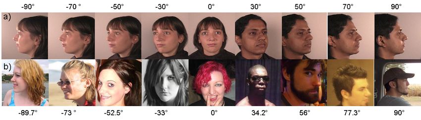
2 AGHAJANIAN, PRINCE: FACE POSE ESTIMATION
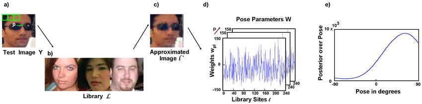
Figure 1: (a) Most of current methods estimate pose in a limited range or treat pose as a
classification problem by assigning the face to one of many discrete poses. Moreover they
have mainly been tested on images taken in controlled environments e.g. with solid/constant
background, with small or no variation in illumination and expression. (b) We address the
problem of estimating pose as a continuous regression problem on “real world” images with
large variations in background, illumination and expression.
on finding the position of facial features, or fitting a tailor made template to the face which
itself is a difficult problem. They also require reliable registration of faces.
Manifold learning approaches consider the high dimensional feature space of face pose as
a set of geometrically related points lying on a low dimensional smooth manifold. They use
linear/non-linear embedding methods to learn this lower dimensional space from the training
data. Pose is then estimated in this space. Several general linear embedding methods such
as PCA [25] and ICA [19], have been proposed. One limitation of these methods is that they
can only recover the true structure of linear manifolds, while the geometry of view-varying
face manifold can be highly folded in the high-dimensional input space.
Alternatively non-linear embedding such as Isomap [4], Local Embedded Analysis (LEA)
[12] and Local Linear Embedding (LLE) [4, 26], have been tried to project the data onto a
lower dimensional non-linear manifold. Pose is then estimated using K-nearest neighbor
classification [12], or multivariate linear regression [4]. These methods are limited in that
the non-linear projection is defined only on the training data space. For each novel input (test
data) the entire embedding procedure has to be repeated or other techniques like Generalized
Regression Neural Networks [4] need to be designed to do this mapping for test data.
One of the limitations of current methods is that most of them estimate pose in a limited
range and treat pose estimation as a classification problem by assigning the face to one of
many discrete poses [17, 18, 19]. However pose estimation is truly a regression problem.
Consider a human computer interaction scenario where we are interested in finding the gaze
direction of the user; it is much more desirable to have a continuous estimation of the head
pose rather than specific head angles. Another major drawback of current methods is that
they have mainly been tested on faces taken in controlled environments (there are exceptions
e.g. [13]) i.e. with solid or constant background and small or no variation in illumination
and expression such as the CUbiC FacePix database [20] (Figure 1a). Ideally we should be
able to estimate pose in uncontrolled environments. Unfortunately current methods are not
capable of this partly because it is very difficult to obtain the ground truth for such images.
In this paper we address both problems of obtaining human estimates of pose (as ground
truth) and automatically estimating pose in images taken in uncontrolled environments. First
we collect a large database (tens of thousands) of “real world” images. This database con-
tains faces with pose varying from −90◦ to 90◦ as well as high variation in illumination,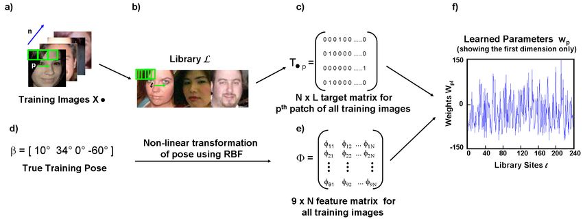
AGHAJANIAN, PRINCE: FACE POSE ESTIMATION                                                      3

Figure 2: Inference. (a) A test image Y is decomposed into a regular patch grid. (b) A large
library L is used to approximate each patch from the test image. (c) The choice of library
patch provides information about the true pose. (d) The model parameters W are used to
interpret these patch choices in a Bayesian framework to calculate a posterior over pose (e).

expression and background clutter (See Figure 1b). We compare our automatically estimated
pose with human estimates of face pose in these real world scenarios.
    We propose a probabilistic framework for continuous pose estimation. Unlike current
methods that have tailor made representations we use a general representation that does not
rely on locating facial features or fitting a model to the face. Instead we represent a face
with a non-overlapping grid of patches. Our approach is inspired by recent successes of
patch-based approaches which have shown to be highly effective for texture generation and
synthesis [9, 23], super-resolution [11], face recognition [2] and within-object classification
[3]. We use this representation in a generative model for automatic estimation of head pose.

2    Methods

Our approach breaks the test image into a non-overlapping regular grid of patches. Each is
treated separately and provides independent information about the true pose. At the core of
our algorithm is a predefined library of object instances. The library can be considered as a
palette from which image patches can be taken. This is similar to the bag of words model
[8]: the library can be thought of as a structured set of textons which are used to quantize
the image patches. We exploit the relationship between the patches in the test image and the
patches in the library to estimate the face pose. Our algorithm can be understood in terms of
either inference or generation and we will describe each in turn.
    In inference (see Figure 2), the test image patch is approximated by a patch from the
library L . The particular library patch chosen can be thought of as having a different affinity
with each pose. These affinities are learned during a training period and are embodied in a
set of parameters W. The relative affinity of the chosen library patch for each pose is used
to determine a posterior probability over pose.
    Alternatively, we can think about generation from this model. For example, consider the
generative process for the top-left patch of a test image. The true pose induces a probability
distribution over all the patches in the library based on the learned parameters W. We choose
a particular patch using this probability distribution and add independent Gaussian noise at
each pixel to create the observed data. In inference we invert this generative process using
Bayes’ rule to establish which pose was most likely to be responsible for the observed data.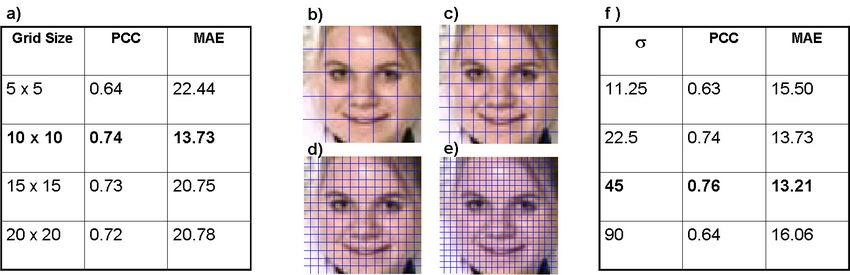
4                                            AGHAJANIAN, PRINCE: FACE POSE ESTIMATION

Figure 3: (a) The model is trained from N training images, each of which is represented
as a non-overlapping grid of patches indexed by p. (b) The library L is considered as a
collection of patches Ll where l indexes the L possible sites. (c) We use 1-of-L coding
scheme to represent the closest library patch lˆ and store them in a target matrix Tp for the pth
patch of all training images. (d) The true poses are stored in a N × 1 vector β . (e) Columns
of Φ represent φ n : 9D radial basis functions of pose parameter β for the nth training image.
(f) We learn the parameter vector wpl which represents the tendency for the library site l to
be picked when considering patch p of an image with pose vector φ n .

2.1    Inference
Consider the task of estimating a continuous value for the pose parameter β for a test image,
where β can have values ranging from −90◦ to 90◦ . The test image Y is represented as a
non-overlapping grid of patches Y = [y1 ...yP ]. The model will be trained from N training ex-
amples X with labeled poses. Each training example is also represented as a non-overlapping
grid of patches of the same size as the test data. We denote the pth patch from the nth training
example by xnp (see Figure 3a).
    We also have a library L of images that are not in the training or test set and would
normally contain examples with various poses. We will consider the library as a collection
of patches Ll where l ∈ {1..L} indexes the L possible sites from which we can take library
patches (see Figure 3b). These patches are the same size as those in the test and training
images but may be taken from anywhere in the library (i.e. they are not constrained to come
from a non-overlapping grid).
    The output of our algorithm is a posterior probability over the pose parameter β . We
calculate this using Bayes’ rule
                                           ∏Pp=1 Pr(y p , l ∗ |β , w p• )Pr(β )
                         Pr(β |Y, W) =                                                           (1)
                                                       Pr(Y)

where we have assumed that the test patches y p are independent. The term β represents pose,
w p• are the parameters of the model and the variable l ∗ is the site in the library that most
closely matches the test patch y p . The notation • indicates all of the values that an index can
take, so w p• denotes the parameter vector associated with the pth patch in the test image and
all of the sites in the library. To find the site l ∗ in the library we assume that the test patch is
a Gaussian corruption of the library patch and use
                                    l ∗ = arg max Gy p [Ll ; σ 2 I]                              (2)
                                              l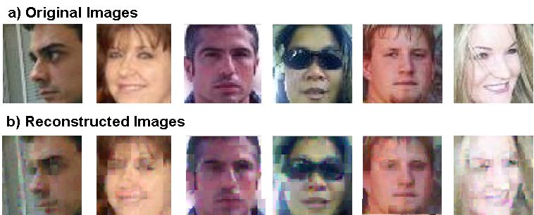
AGHAJANIAN, PRINCE: FACE POSE ESTIMATION                                                              5

where Ll is the patch from site l of the library L .
    We now define the likelihood in Equation 1 to be a multinomial distribution on the library
sites. The model takes the form of a multi-class logistic regression where the classes are the
library sites and the data variable is the pose vector φ :
                                                            exp(w pl ∗ T φ )
                             Pr(y p , l ∗ |β , w p• ) =    L
                                                                                                     (3)
                                                          ∑l=1 exp(w pl T φ )
where φ = {φ1 ..φJ } is chosen to be 9D radial basis functions (RBF) defined as
                                                           !
                                               (β − µ j )2
                                  φ j = exp −                                                        (4)
                                                  2σ 2

where j ∈ {1..9} and µ j govern the locations of the basis functions in input space and lie
within −90◦ to 90◦ . The term σ denotes the standard deviation and is set during training
(See Figure 3e). The parameter w pl represents the tendency for the patch from library site l
to be picked when considering patch p of an example image with pose vector φ . This can be
visualized as in Figure 3f. To find the best pose we do a one dimensional line search on pose
varying from −90◦ to 90◦ and estimate the pose by maximizing the energy function that is
set to be the posterior probability over pose i.e. Pr(β |Y, W) in Equation 1.

2.2    Training
In this section, we consider how to use the training data x•p from the pth patch of all of the
N training images to learn the relevant parameters wp• = {w p1 ..w pL } where L is the size of
the library. Notice we learn a separate weight vector w p• for each patch in the input image.
This is done by maximizing the likelihood of the observed patches in the training images
given their poses with respect to the parameters w p• . This procedure is similar to multi-class
logistic regression (See [5] for more details). The likelihood of a single training patch xnp
from the nth training image is defined as:
                                                                     exp(w plˆT φ n )
                      znplˆ(φφ ) = Pr(x p , lˆn |β , w p• ) =                                        (5)
                                                                ∑Ll=1 exp(w pl T φ n )

where lˆn is the library site that most closely matches the training patch xnp and is defined as

                                    lˆn = arg max Gxnp [Ll ; σ 2 I]                                  (6)
                                               l

    Now we will use 1-of-L coding scheme to represent the selected library site lˆn for each
patch of each training image and store it in a target vector tnp . Thus, tnp is the target vector
for the pth patch of the nth training example with a feature vector φ n , and is a binary vector
with all elements zero except for lˆn which equals one. Now consider the entire training data,
we can now rewrite the likelihood term in Equation 5 as follows:

                                                      N     L                                tnpl
                   Pr(T•p |w p1 , ..., w pL ) =      ∏ ∏ Pr            xnp , lˆn |β , w p•           (7)
                                                     n=1 l=1
                                                      N L
                                                          npl    t
                                               =     ∏ ∏ znpl
                                                     n=1 l=1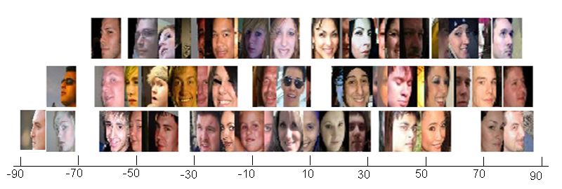
6                                             AGHAJANIAN, PRINCE: FACE POSE ESTIMATION

Figure 4: Some example images along with the average human estimate of pose. The x-axis
represents the average labeled pose which is used as the ground-truth.

where znpl = z pl (φφ n ) and T•p is a N × L matrix of target vectors (closest library sites) for pth
patch and all of the training images with elements tnpl (See Figure 3c). Taking the negative
logarithm of Equation 7 then gives
                                                                        N      L
               E(w p1 ...w pL ) = − ln Pr(T•p |w p1 , ..., w pL ) = − ∑     ∑ tnpl ln znpl       (8)
                                                                       n=1 l=1
    We now minimize the negative log-multinomial likelihood (Equation 8) to determine the
parameters w pl . This is done by taking the gradient of Equation 8 with respect to one of the
parameter vectors w pl (for details on the derivatives of the softmax function see [5]). After
this procedure we obtain:
                                                        N
                             ∇w pl E(w p1 ...w pL ) =   ∑ (znpl − tnpl )φφ n                     (9)
                                                        n=1

where we made use of ∑Ll=1 tnpl = 1. Because Equation 8 depends on all of the parameters
w p1 ...w pL we concatenate all ∇w pl to from the derivative and repeat for every patch.

3    Dataset
We harvested a large database of images of men and women from the web. These were
captured in uncontrolled environments and exhibit wide variation in illumination, scale, ex-
pression and pose as well as partial occlusion and background clutter (see Figure 1b). Faces
were detected using a commercial frontal face detector [1] to automatically find face regions.
The images were subsequently transformed to a 60x60 template using a Euclidean warp. We
band-pass filtered the images and weighted the pixels using a Gaussian function centered on
the image. Each image was normalized to have zero mean and unit standard deviation.
    To obtain a human estimate of pose for the above dataset, four subjects were asked to
label the pose in face images ranging from −90◦ to 90◦ in 10◦ steps. The subjects were
shown relevant images from the CUbiC FacePix database [20] as a reference and asked to
label the images according to their similarity to the pose in the reference image. Due to the
large number of images the dataset was divided into two subsets. Two different subjects were
asked to label each subset of the data separately. The labeled poses of the two subjects were
averaged to obtain a continuous estimate of pose for that subset. Some example images with
their average labeled pose are shown in Figure 4. The x-axis represents the average labeled
pose which is used as average human estimate. However, the obtained human estimate is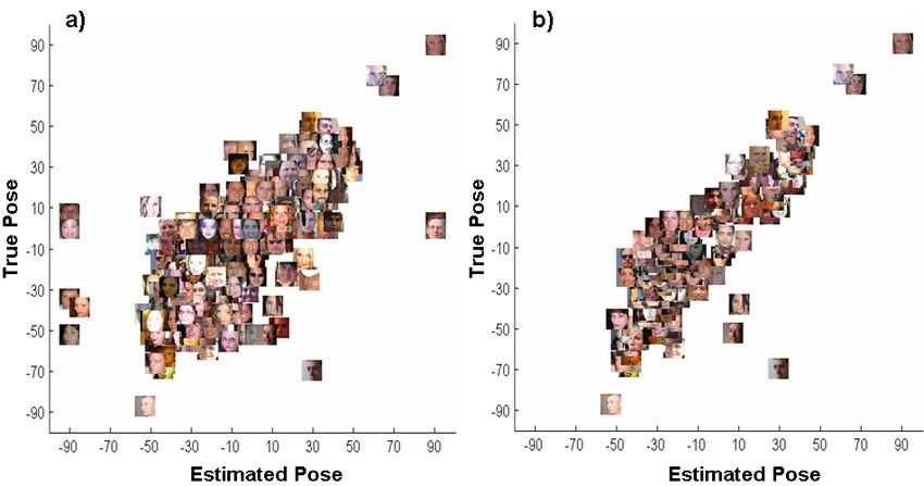
AGHAJANIAN, PRINCE: FACE POSE ESTIMATION                                                        7

Figure 5: (a) The distribution of poses in training and test data. (b) The proportion of the test
data that lies within an error range in degrees. (c) The cumulative population of the data as a
function of the pose error in degrees for hand labeled poses (red) and our method (blue). We
observe that with our method around 87% of the test data have an error of 20 degrees or less
which is equivalent to the error between two subjects in hand labeled poses.

still considered noisy since the poses labeled by the two subjects only have a correlation
coefficient of 0.76 on the training set and 0.73 on the test set. To measure the noise level in
the human pose estimate we plot the cumulative population of the test data as a function of
the mean absolute error (MAE : the absolute error averaged across all test images) between
the two subjects. This is shown in Figure 5c, and results in a MAE of 10.89 degrees.

4    Experiments
We test our algorithm on automatic pose estimation given the unconstrained face images. In
this experiment we used 10,900 training images and 1000 test images. The library is made
up 240 images similar to [3]. The training, testing and library sets are randomly selected,
are non-overlapping and contain poses varying from −90◦ to 90◦ . Note that since we used
a commercial frontal face detector to automatically locate the faces, some of the faces with
large pose angles might have been missed hence we do not have an even distribution of poses
in our dataset. The pose distribution for training and test set are shown in Figure 5a.
    We investigate the effects of two parameters on the performance of our algorithm on pose
estimation: (i) the patch grid resolution and (ii) the standard deviation σ of the radial basis
functions. We measure the performance of our algorithm using the following metrics: (i)
Pearson correlation coefficient (PCC) between the true pose and the estimated pose and (ii)
mean absolute error (MAE): which is the absolute error averaged across all test images.
    In the first experiment we vary the grid resolution from 5 × 5 to 20 × 20 by keeping
the standard deviation fixed at σ = 22.5. The results are summarized in Table 6a. The
performance peaks at 10 × 10 grid (6×6 pixels). We achieve a correlation coefficient of 0.74
between the true and estimated pose on the test set with a MAE of 13.75. For visualization
purposes we also plot the patch grid on a sample face in Figure 6(b-e) for 5 × 5, 10 × 10,
15 × 15 and 20 × 20 grid sizes respectively. It can be seen that as the grid resolution becomes
higher the patches themselves become very small and perhaps not very informative for the
task. To further verify that 6×6 pixel patches in the 10×10 grid are sufficient we reconstruct
the original images using the closest patches l ∗ from the library (see Figure 7). To find the
closest library patch l ∗ in a computationally efficient way, in practice we restrict the possible
indices l to a subset corresponding to a 6 × 6 pixel window around the current test patch
position in each library image so patches containing eyes are only approximated by other
8 AGHAJANIAN, PRINCE: FACE POSE ESTIMATION
Figure 6: (a) Comparison of performance on pose estimation in various grid resolutions with
fixed σ = 22.5, measured by Pearson correlation coefficient (PCC) and mean absolute error
in degrees (MAE) between the true pose and the estimated pose. Visualization of (b) 5 × 5
(c) 10 × 10 (d) 15 × 15 and (e) 20 × 20 grid sizes. (f) Comparison of performance on pose
estimation on various values of σ with patch grid resolution fixed at 10 × 10.
Figure 7: We verify that 6 × 6 pixel patches are sufficient by reconstructing the original
images using the closest patches l ∗ from the library. It is still easy to identify the pose of the
images using the approximated versions. Note: for illustration purposes the RGB form of
the test and library images were used in this case to produce the reconstructed images above.
patches containing eyes etc. Figure 7 shows that it is still easy to identify the pose of the
images using the approximated versions therefore it is fair to assume that the 6 × 6 patches
have preserved the pose related information contained in the face images.
In the second experiment we vary the overlap between the 9D radial basis function i.e.
the term σ in Equation 4 by keeping the patch grid resolution fixed at 10 × 10. We test our
algorithm with three different values for σ : 11.25 , 22.5, 45 and 90 degrees. The results of
this experiment are summarized in Figure 6f. The results demonstrate change as the overlap
between the radial basis function is varied, reaching a peak with σ = 45 where we achieve
a correlation coefficient of 0.76 on the test data with a MAE of 13.21. The scatter plot of
the results on 10 × 10 grid with σ = 45 is shown for all of the test data in Figure 8a, and for
a subset of the test data uniformly sampled from each true pose in Figure 8b. We achieve a
higher PCC of 0.88 for the uniformly sampled test set with a lower MAE of 11.72. We also
plotted the proportion of the test data that lies within an error range in degrees (Figure 5b)
as well as the cumulative population of the data as a function of the pose error in degrees
(Figure 5c). We observe that around 87% of the test data have an error of 20 degrees or less.AGHAJANIAN, PRINCE: FACE POSE ESTIMATION 9
Figure 8: Scatter plot of the results on 10 × 10 grid with 9D RBF and σ = 45 (a) for all of the
test data. We achieve a PCC of 0.76 and a MAE of 13.21 degrees and (b) for a subset of the
test data uniformly sampled at each true pose. We achieve a PCC of 0.88 and a MAE of 11.72
degrees. The x-axis and y-axis represent the estimated pose and the true pose respectively.
5 Summary and Discussions
In this paper we have proposed a probabilistic framework for automatic estimation of pose
as a regression problem. Our algorithm uses a generic patch-based representation and does
not rely on object-specific landmarks, therefore it can be used for regression problems on
other object-classes without major alterations. We demonstrate good performance on ‘real
world’ images of faces with poses varying from −90◦ to 90◦ . The algorithm has a close re-
lationship with nonparametric synthesis algorithms such as image quilting [9] where patches
from one image are used to model others. Our algorithm works on similar principles - all the
knowledge about the object class is embedded in the library images. This accounts for why
the algorithm works so well in different circumstances. If we have enough library images
they naturally provide enough information to discriminate the classes.
Unfortunately it is not easy to compare our algorithm with other methods such as support
vector machines and manifold learning methods, because they cannot usually handle such
large datasets and have mostly been tested on controlled databases. Current methods achieve
various results based on whether classification or regression approach was used, as well as
the particular database used. The results typically vary between a MAE of around 7.84 de-
grees with SVR [14] and 59.91 degrees using kernel SVM [14] on the Pointing’04 database
and between around 2 to 12 degrees using Biased Manifold Embedding [4] on the CUbiC
FacePix database (correlation coefficients are not available). Note that despite their high per-
formance, it is not easy to see how these methods will generalize on unconstrained databases
such as the one used in this paper. We achieve an MAE of 11.72 and a PCC of 0.88 on a
uniformly sampled database of “real world” images which is comparable to the performance
of other methods tested on controlled databases. Remarkably the PCC of our algorithm to
average human performance is about the same as the PCC of two human subjects. This
suggests that our performance is limited by the fidelity of the original labelling.
In terms of scalability our algorithm is linear with respect to the size of the library and
the dimension of the RBF function. We perform a non-linear optimization to estimate the10 AGHAJANIAN, PRINCE: FACE POSE ESTIMATION
parameters W where we have used the method of BFGS Quasi-Newton. For a library of size
m and a n dimensional RBF function, for each patch the processing time scales as O(mn) in
training and O(n) in testing.
In future work we would like to improve the accuracy of the ground-truth by using land-
marks along with other regression mechanisms such as support vector regression similar to
[21]. We also intend to investigate other visual tasks such as localization and segmentation
using similar methods that exploit a library of patches and a large number of training images.
Acknowledgements We acknowledge the support of the EPSRC Grant No. EP/E013309/1.
We would also like to thank Ashley Harris, Mateusz Manikowski, Tomas Majersky and Yun
Fu for their kind help with labeling poses.
References
[1] A. Konoplev. Luxand FaceSDK.
[2] J. Aghajanian and S.J.D. Prince. Mosaicfaces: a discrete representation for face recog-
nition. In WACV, pages 1–8, 2008.
[3] J. Aghajanian, J. Warrell, S.J.D. Prince, J.L. Rohn, and B. Baum. Patch-based Within-
Object Classification. In ICCV, 2009.
[4] VN Balasubramanian, J. Ye, and S. Panchanathan. Biased Manifold Embedding: A
Framework for Person-Independent Head Pose Estimation. In CVPR, pages 1–7, 2007.
[5] C.M. Bishop. Pattern Recognition and Machine Learning (Information Science and
Statistics). pages 205–210, 2006.
[6] M.D. Breitenstein, D. Kuettel, T. Weise, L. Van Gool, and H. Pfister. Real-time face
pose estimation from single range images. In CVPR, pages 1–8, 2008.
[7] K.N. Choi, M. Carcassoni, and E.R. Hancock. Estimating 3D facial pose using the EM
algorithm. Face Recognition: From Theory to Applications, pages 412–423, 1998.
[8] G. Csurka, C. Dance, L. Fan, J. Willamowski, and C. Bray. Visual categorization with
bags of keypoints. In Workshop on Statistical Learning in Computer Vision, ECCV,
volume 1, page 22, 2004.
[9] A.A. Efros and W.T. Freeman. Image quilting for texture synthesis and transfer. In
SIGGRAPH, pages 341–346, 2001.
[10] E. Elagin, J. Steffens, and H. Neven. Automatic pose estimation system for human
faces based on bunchgraph matching technology. In AFGR, pages 136–141, 1998.
[11] W.T. Freeman, E.C. Pasztor, and O.T. Carmichael. Learning low-level vision. In IJCV,
volume 40, pages 25–47, 2000.
[12] Y. Fu and TS Huang. Graph embedded analysis for head pose estimation. In AFGR,
page 6, 2006.
[13] N. Grujic, S. Ilic, V. Lepetit, and P. Fua. 3d facial pose estimation by image retrieval.
In AFGR, 2008.AGHAJANIAN, PRINCE: FACE POSE ESTIMATION 11
[14] G. Guo, Y. Fu, C.R. Dyer, and T.S. Huang. Head pose estimation: Classification or
regression? In ICPR, pages 1–4, 2008.
[15] J. Heinzmann and A. Zelinsky. 3-D facial pose and gaze point estimation using a robust
real-time tracking paradigm. In AFGR, pages 142–147, 1998.
[16] Y. Hu, L. Chen, Y. Zhou, and H. Zhang. Estimating face pose by facial asymmetry and
geometry. In AFGR, pages 651–656, 2004.
[17] N. Kruger, M. Potzsch, T. Maurer, and M. Rinne. Estimation of face position and pose
with labeled graphs. In BMVC, pages 735–743, 1996.
[18] SZ Li, Q. Fu, L. Gu, B. Scholkopf, Y. Cheng, and H. Zhang. Kernel machine based
learning for multi-view face detection and pose estimation. In ICCV, volume 2, 2001.
[19] SZ Li, X.H. Peng, X.W. Hou, H.J. Zhang, and Q.S. Cheng. Multi-view face pose
estimation based on supervised isa learning. In AFGR, pages 100–105, 2002.
[20] G. Little, Krishna S., Black J., and Panchanathan S. A methodology for evaluating
robustness of face recognition algorithms with respect to changes in pose and illumi-
nation angle. In ICASSP, 2005.
[21] Y. Ma, Y. Konishi, K. Kinoshita, S. Lao, and M. Kawade. Sparse bayesian regression
for head pose estimation. In ICPR, 2006.
[22] Y. Matsumoto and A. Zelinsky. An algorithm for real-time stereo vision implementa-
tion of headpose and gaze direction measurement. In AFGR, pages 499–504, 2000.
[23] U. Mohammed, S.J.D. Prince, and J. Kautz. Visio-lization Generating Novel Facial
Images. In SIGGRAPH, 2009.
[24] L.P. Morency, P. Sundberg, and T. Darrell. Pose estimation using 3d view-based
eigenspaces. In AMFG, pages 45–52, 2003.
[25] K. Okada, S. Akamatsu, and C. Von der Malsburg. Analysis and synthesis of pose vari-
ations of human faces by alinear PCMAP model and its application for pose-invariant
facerecognition system. In AFGR, pages 142–149, 2000.
[26] B. Raytchev, I. Yoda, and K. Sakaue. Head pose estimation by nonlinear manifold
learning. In ICPR, volume 4, 2004.
[27] J.G. Wang, E. Sung, and R. Venkateswarlu. Determining pose of a human face from a
single monocular image. In BMVC, 2003.
[28] Y. Zhou, L. Gu, and H.J. Zhang. Bayesian tangent shape model: Estimating shape and
pose parameters via bayesian inference. In CVPR, volume 1, 2003.You can also read