Assessment of Machine Learning of Optimal Solutions for Robotic Walking - ijmerr
←
→
Page content transcription
If your browser does not render page correctly, please read the page content below
International Journal of Mechanical Engineering and Robotics Research Vol. 10, No. 1, January 2021
Assessment of Machine Learning of Optimal
Solutions for Robotic Walking
Rodrigo Matos Carnier and Yasutaka Fujimoto
Yokohama National University, Yokohama, Japan
Email: Rodrigo.carnier@gmail.com, fujimoto@ynu.ac.jp
Abstract— The generation of optimal solutions for robotic prototypes that are able to perform complex human tasks
bipedal walking using whole-body dynamics is well known and interact with humans, like Atlas [2], HRP-5P [3] and
to have a big computational cost, preventing online ASIMO [4]. However, the best prototypes in the world
trajectory generation for optimal control methods that nowadays are still nowhere near the level of performance
satisfy Pontryagin's Principle and its Conditions of
of human beings [5] [6]. Controlling such an
Optimality. However, bipedal walking has fundamental
kinematic and dynamic characteristics that shape different underactuated and unstable mechanical task is one of the
solutions for different parameters in similar curves. Such reasons, as well as the advanced optimization achieved by
characteristics were previously defined in biomechanical human evolution while improving different performance
literature as movement primitives. Recently, studies criteria at the same time (e.g. speed of reflexes and
generated parametrized optimal solutions by performing energy expenditure). Since evolution is a form of
regressions from training data into movement primitives optimization and the human gait is the natural inspiration
using Machine Learning. The learned solutions were very for robotic walking, Optimal Control is becoming a
close to the actual optimal solution. This study evaluates the natural choice for improvement of performance, but it
precision of such strategy by optimizing the gait of a 6
cannot yet perform very well in real time. Therefore,
degrees of freedom planar robot using different Cost
Functions, in order to understand if the precision of optimal solutions for the locomotion of biped robots are
Machine Learning in recreating optimal solutions is either online but imprecise, or precise but offline.
impacted by what is being optimized. Another way of improving walking performance is
applying Machine Learning to extract better solutions
Index Terms— robotic bipedal walking, machine learning, from experience and repetition. This has been done for
optimal control, movement primitives several different purposes, from decision making of when
to step to avoid a fall [7] to the complete gait generation
through Reinforcement Learning [8]. Another interesting
I. INTRODUCTION approach is to reproduce the performance of Optimal
Optimal Control is a field of study that has become Control by generating new optimal solutions from a set of
popular in the last 20 years. Even though its mathematical training optimal solutions without reproducing the whole
theory was developed more than 60 years ago, it started optimization process. Solutions generated this way can be
to be widely investigated only with the advent of greatly produced very fast, partially circumventing the problems
increased computational power in the beginning of 2000's of real time complex optimization. Recently, this has
[1]. Consequently, many challenges remain, including the been done by extracting movement primitives from
realization of proper optimization (in contrast to optimal solutions [9] [10]. Movement primitives are
suboptimization) in real time. While most current fundamental kinematic and dynamic characteristics
implementations of online optimization only decrease a shared by different solutions of specific classes of
Cost Function, proper optimization satisfies the movements (like walking, running, jumping or grasping).
Conditions of Optimality defined by Pontryagin's Given a body morphology (e.g. the human or the avian
Principle or its equivalents (e.g. Hamilton-Jacobi- body morphology), the shape of the curve of a solution
Bellman Equation). However, the computational cost of for bipedal walking is just slightly changed depending on
solving an optimization problem satisfying these the parameters of movement (like body mass, length of
conditions is still critically high for nonlinear systems body limbs, speed of movement, distance traversed).
with many degrees of freedom and very dynamic Based on this, Koch et al. [10] extracted movement
behavior – in other words, systems with dynamics primitives from optimal solutions for bipedal walking
changing in the milliseconds, needing to be controlled in through Principal Component Analysis, parametrized the
such a timespan. MP according to step size of walking and then performed
Robotic bipedal walking is one of such fields. Inspired a stochastic regression by Gaussian Process to generate
in the locomotion of human beings, it has come a long new solutions very close to the actual optimal solution.
way in its 50 years or so of life, generating impressive The present study investigates the precision of such
approach. Koch et al. [10] investigated only the learning
of optimal solutions minimizing the square of torques
Manuscript received March 14, 2020; revised November 1, 2020.
© 2021 Int. J. Mech. Eng. Rob. Res 44
doi: 10.18178/ijmerr.10.1.44-48
International Journal of Mechanical Engineering and Robotics Research Vol. 10, No. 1, January 2021
applied on joints. In the present study we will confront
the results of minimization of torques with the (2)
minimization of energy consumption, modelled as
friction in the joints. In the sequence of this introduction,
we will describe the dynamics of the model, the optimal III. OPTIMAL CONTROL PROBLEM
control problem formulation, the learning methodology The optimal control method used in this study is a
used and the gait synthesis of our biped model. An pseudospectral method based on the Pontryagin's
evaluation of success of the machine learning method Principle and the Covector Mapping Theorem [1]. The
will be explained in the last section, together with a method relies on discretizing the system and minimizing
discussion of the results. the control Hamiltonian of the system in order to achieve
the optimal solution.
II. DYNAMICS In this work, we optimized two different cost functions:
The model used for studying the optimization of biped minimization of actuators efforts and minimization of
walking is a planar model of robot with 6 DOF. Control energy consumption. These optimizations were
of walking is performed only in the sagittal plane. The performed independently of each other. For each one, a
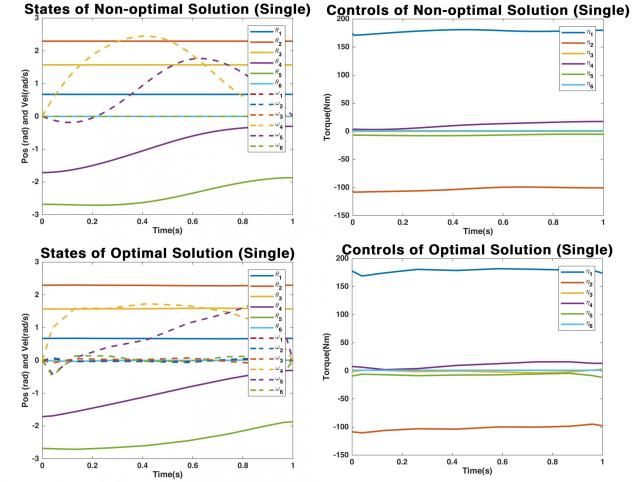
model is treated as a manipulator fixed in the ground (Fig. different analytic formulation of cost was used:
1), since a model with the ankle of the support foot fixed 1. Minimization of Actuators Efforts: A common
to the floor can be considered equivalent to a free floating objective of optimization in robotics is the
robot model as long as the forces and torques applied by generation of smooth controls. This can be done
the floor to the fixed foot never pull it to the floor, nor by minimizing the square of torques applied in the
take the Zero-Moment Point [11] away from the base of joints .
support of the robot. 2. Minimization of Energy Consumption: In our
dynamic model, energy loss is modeled as viscous
friction in the joints ( ), which is propor-
tional to the joint angular velocities ( ). The
optimization is performed by minimizing the
square of friction .
In both costs, joint quantities are being used ( and ).
However, our dynamic formulation was based on links
reference. To maintain reference coherence, and_ are
expressed in terms of η and through the transformations
below:
Figure 1. Planar model with 6 DOF, with representation of link angles.
(3)
The system states are the absolute angular position and where G and K are transformation matrixes that depend
the angular velocity of the robot links. The position is on the kinematic chain of the robot.
represented by θ and is measured in respect to the The minimization of torques is then defined as an
horizontal axis (x) of the world reference, fixed outside objective of optimization by (4), while the minimization
the robot. The dynamics of the mechanical system is of friction is defined by (5).
derived in the usual way from its Euler-Lagrange
Equations [12]: (4)
(1)
(5)
where M is the Total Inertia matrix, B is the Coriolis and
centrifugal effects, C is the friction acting on joints, G is With these definitions, we solved the optimal
the gravitational effect, η is the internal torques working trajectory generation of model of Fig. 1 using the
on the links by joint actuators, J is the jacobian of the commercial optimal solver DIDO. It is necessary to
external forces applied on the end-effector by contact provide three different elements to the solver: 1) the
with the ground, and R is the ground reaction forces. analytic expressions of the system dynamics, of the cost
If we group the two vectors of states – angle of links function J and of any path constraints (floor contact
and angular velocity of links – in a single vector of states, constraints, in our case); 2) the boundaries for the search
we obtain the following concise formulation of the space of states, controls and constraints; and 3) the
system dynamics in state-space: desired initial and final value of states. In our case, these
initial and final states represent the initial and final stance
© 2021 Int. J. Mech. Eng. Rob. Res 45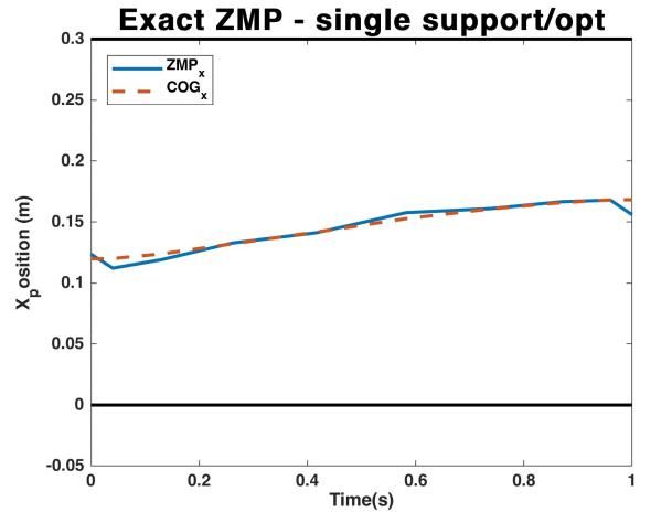
International Journal of Mechanical Engineering and Robotics Research Vol. 10, No. 1, January 2021

of the bipedal robot model. DIDO then generates                        as training data, in order to only change the value of the
trajectories for the states and controls, which bring the              parameter to obtain new solutions.
robot from the initial stance to the final stance, making                 The method of Machine Learning applied in this study
the robot take a step. A detailed description of our                   is Gaussian Process. It is a probabilistic type of
methodology for solving such a nonlinear multidegree-of-               regression based on gaussian distributions and differ from
freedom system is given in Carnier and Fujimoto [13].                  deterministic regressions by adding flexibilization to the
   For more details on DIDO or its pseudospectral                      learning process and allowing incremental improvement
method, refer to Ross [14] [15] or Ross and Fahroo [16].               of learning experience.
                                                                          For comparison sake, take the deterministic types of
                 IV.     MOVEMENT PRIMITIVES                           regression: these simpler regressions are based on taking
                                                                       observed points to find a function or curve that can
   Given a mechanical walking system with its
                                                                       approximate the points. This can be done minimizing an
morphology, parameters and constraints, the variability of
                                                                       error function between the parametrized function on a
kinematic and dynamic trajectories for the states of the               time instant and the observed point on the same instant
system are restricted to a fundamental dynamic behavior,               (e.g. least square root of distance between observation
which can be expressed as proto-trajectories called
                                                                       points and function points). In other words, the regression
movement primitives. This similar dynamic behavior in
                                                                       process consists of calculating the function parameters
different walking solutions can be observed in the same                that make the approximate function fit the observed
shape of its state and control trajectories. Which dynamic             points best. The resulting function then can be used to
properties are present in the movement primitive and
                                                                       predict new points.
which are not, depends on the training set of solutions
                                                                          A probabilistic type of regression creates instead a
used to extract the movement primitive. If a set of                    probabilistic distribution that best describes the likelihood
optimal solutions is used, the property of optimality can              of new data matching the observed behavior. Like
possibly be extracted.
                                                                       deterministic regressions, it creates a form of
   The process is done as follows: first we generate a
                                                                       parametrization of the observed data that can be used to
number Nsol of solutions for different values of a given               predict new information. But unlike deterministic
parameter, which in our case is the length of walking step.            regressions, it takes uncertainty of data into account and
Each solution has NDOF trajectories of link angles, each
                                                                       give more tools to work around it.
with Nt points of discretization. Then, we group all these
                                                                          First, uncertainty is accounted for in the calculation of
time-series trajectories of link angles into a single matrix           a learned model. Instead of representing a deterministic
X of size (Nsol NDOF) × Nt. In our case, X has a size of 48            function, it represents a gaussian distribution that
× 15. The extraction of the movement primitive is done
                                                                       maximizes its marginal log-likelihood of reproducing the
by performing a Single Value Decomposition (SVD) of X.
                                                                       observed data (in other words, the parameters of
According to Principal Component Analysis theory, SVD                  distribution that makes the most probable point of
extracts eigenvalues of the Principal Component of a set               distribution – the mean – closest to the observation
of solutions, which in our case is the essential dynamics
                                                                       points). The probabilistic regression method used in this
of an optimal solution of biped gait. SVD extracts the
                                                                       study – Gaussian Process – further exploits the uncertain-
three following matrixes:                                              ty to improve the regression. Since the uncertainty of
                         [U, S, V] = SVD (X)                (6)        regression is dependent on the quantity and variability of
                                                                       initial observed data used to generate the parametrized
   The movement primitive then is calculated from these                distribution, Bayes' Theorem is used to improve the
terms according to (7):                                                certainty of regression by allowing new observations to
                               M=SVT                        (7)        be inserted into the regression, in order to expand it. In
                                                                       this way, an initial regression can be improved over time,
   These matrixes represent the following information:                 by simply decreasing its uncertainty instead of
   1. M: the movement primitive.                                       performing a new regression. Much like biological agents
   2. U: a matrix of weights that multiply the movement                evolve and expand their experience to improve their
       primitive in order to generate one or more                      performance.
       solutions. This matrix U in particular is the matrix               To machine learn the new solutions with different
       of original weights, that will regenerate X if we               parameters, first a gaussian regression model needs to be
       perform the multiplication UM.                                  extracted from the training optimal trajectories. This is
                                                                       done by performing n model regressions:
                    V.    MACHINE LEARNING
                                                                                                n = NDOF NMP                     (8)
   Machine Learning is a broad definition of many
techniques that take a training set of information, solution           where NMP is the number of movement primitives (i.e. the
or decision and extract a structure able to make                       number of lines of matrix M). Since our model has 6
predictions of the same sort. In very simplified sense,                DOF and the chosen number of movement primitives is 5,
Machine Learning is a much more abstract version of                    a total of 30 elements need to be learned for each new
equation regression. For our purposes, Machine Learning                optimal solution we desire to generate through Machine
is used to parametrize the set of optimal solutions taken              Learning. The routine fitrgp implemented in MATLAB is

© 2021 Int. J. Mech. Eng. Rob. Res                                46
International Journal of Mechanical Engineering and Robotics Research Vol. 10, No. 1, January 2021

used for this regression. Since the different training
solutions were used varying the parameter of size of
stride in gait, this parameter is given as input of the
parametrized regression.
   After learning the model, new solutions for different
parameters are generated by maximizing the marginal
log-likelihood of the regression model for a solution with
a new desired stride length. This is done through routine
predic, also implemented in MATLAB.
   General details of the followed methodology can be
found in Koch et al. [10].

                     VI.    IMPLEMENTATION
   The robot model was designed with parameters
equivalent to a human of average size. It had 1.35m of
height and 48kg of mass distributed in its links (the torso                  Figure 3. Trajectory of states and controls for minimization of friction.
                                                                                     Top: non-optimal solutions. Bottom: optimal solutions.
concentrated most of its mass, at 38kg). During gait the
hip was kept constant at 0.5m, and initial and final
velocities of all links were zero. The gait of this model
                                                                                          VII.    MACHINE LEARNING RESULTS
was designed to satisfy the classic Zero-Moment Point
(ZMP) criterion. The ZMP trajectory of our optimized                            The direct evaluation of success of the methodology is
gait is shown in Fig. 2.                                                     the calculation of the Cost Functions (4) and (5) for the
                                                                             non-optimal solution, machine learned solution and
                                                                             optimal solution. The results are given in Table I.

                                                                             TABLE I.      COST FUNCTIONS OF MACHINE LEARNED, NON-OPTIMAL
                                                                                                  AND OPTIMAL SOLUTIONS

                                                                                   Solution                      Cost Function
                                                                                                      Torque (Nm)2          Friction (Nm)2
                                                                                 Non-optimal            2.3466e3                0.7494
                                                                                  Optimal               1.2503e3                0.7149
                                                                                  Learned               1.2496e3                0.7153

                                                                                The results show an improvement (decrease) of costs
                                                                             from optimal to non-optimal solutions of 46.718% for the
                                                                             minimization of torque 4.6038% for the minimization of
                                                                             friction. Even though the optimization of the former
                                                                             seems to be much more successful than of the later, it is
 Figure 2. ZMP trajectory for walking step. Black lines represent the        explained by the difficult in having a big energy
                boundaries of the base of support.                           minimization just by decreasing friction for the same task,
                                                                             while the torque used to swing a leg can vary
   To generate the training data for Machine Learning,                       considerably for the same task with different trajectories.
solutions for 9 different sizes of walking step were                         Therefore, the real evaluation of the methodology of
generated, ranging from 0.4m to 0.8m. From these                             learning optimal solutions by machine learning is done by
solutions, the one for 0.6m of walking step size was set                     verifying the degradation of optimal solution from the
apart for comparison with the machine learned solution                       actual optimized solution to the learned optimal solution.
generated for the same walking step size. In order to                        The degradation is calculated as the percentage increase
evaluate the success of optimization, the non-optimal                        of the Cost from the optimized solution to the learned
solution used as initial guess was also simulated, and its                   solution. For the minimization of torque, it amounts to
data was compared to the data of the optimal solution.                       0.05599%, while for the minimization of friction, to
Details on the generation of the non-optimal solution and                    0.05595%. In other words, there is practically no
of the optimization process can be found in Carnier and                      degradation at all from the actual optimal solutions to the
Fujimoto [13].                                                               learned ones, even with a training set of optimal solutions
   Below, Fig. 3 presents the trajectories of states and                     of only 8 different parameters, with 15 points of
controls for optimal and non-optimal gaits in the case of                    discretization of time.
minimization of friction as described by (5). In the                            The results demonstrate a high ability of replicating the
trajectories of states, full lines represent angular position                performance of optimal solutions with very few training
of links and traced lines represent angular velocity.                        solutions, and confirms the ability of Machine Learning
                                                                             in generating optimal solutions much faster than actually
                                                                             solving the optimization: in less than half a second, in

© 2021 Int. J. Mech. Eng. Rob. Res                                      47
International Journal of Mechanical Engineering and Robotics Research Vol. 10, No. 1, January 2021

comparison to the 40s of computation required by the                                    challenge finals: Results and perspectives,” Journal of Field
                                                                                        Robotics, vol. 34, no. 2, pp. 229-240, 2017.
optimal solver to generate an optimal solution.
                                                                                 [7]    C. Kouppas, Q. Meng, M. King, and D. Majoe, “S.A.R.A.H.: The
                                                                                        bipedal robot with machine learning step decision making,”
                         VIII.    SUMMARY                                               International Journal of Mechanical Engineering and Robotics
                                                                                        Research, vol. 7, no. 4, pp. 379-384, 2018.
   This paper assessed the precision of machine learning                         [8]    C. R. Gil, H. Calvo, and H. Sossa, “Learning an efficient gait
optimal solutions for a planar biped robot model in the                                 cycle of a biped robot based on reinforcement learning and
task of walking. The optimal solutions used as training                                 artificial neural networks,” Applied Sciences, vol. 9, no. 3, 502,
                                                                                        2019.
data were generated by pseudospectral optimization of                            [9]    A. d’Avella and M. C. Tresch, “Modularity in the motor system:
smoothness and of energy consumption in the bipedal                                     Decomposition of muscle patterns as combinations of time-
locomotion of a planar model of robot walker, using its                                 varying synergies,” Advances in Neural Information Processing
whole-body dynamics for precise optimization.                                           Systems, vol. 14, pp. 141-148, The MIT Press, 2002.
                                                                                 [10]   K. H. Koch, D. Clever, K. Mombaur, and D. Endres, “Learning
Movement primitives that contains the core dynamics of                                  movement primitives from optimal and dynamically feasible
biped gait were extraction from a set of optimal solutions                              trajectories for humanoid walking,” in Proc. IEEE-RAS 15th
with different parameters (length of stride) and applied                                International Conference on Humanoid Robots (Humanoids), pp.
Machine Learning to create new optimal solutions from                                   866-873, 2015.
                                                                                 [11]   M. Vukobratovic and B. Borovac, “Zero-moment point - thirty
the movement primitives.                                                                five years of its life,” International Journal of Humanoid Robotics,
   Learned optimal solutions were compared with optimal                                 Vol.1, No.1, pp.157-173, 2004.
solutions generated by actual optimization process. A                            [12]   T. Sugihara, Y. Fujimoto, “Dynamic analysis: Equations of
very small deterioration of only about 0.055% of the Cost                               motion,” in Humanoid Robotics: A Reference, A. Goswami, P.
                                                                                        Vadakkepat, pp.723-754, Springer, 2018.
Value of the optimal solution in respect to the actual                           [13]   R. M. Carnier and Y. Fujimoto, “Numerical techniques for the
optimal solution was observed, confirming the ability of                                optimization of gait generation,” IEEJ Journal of Industry
the methodology in reproducing optimal solutions with a                                 Applications, vol. 10, no. 2, 2021. (Accepted)
decrease of computational time from 40s to less than half                        [14]   A Beginner’s Guide to DIDO: A MATLAB Application Package
                                                                                        for Solving Optimal Control Problems, Elissar Global, 2007.
a second.                                                                        [15]   I. M. Ross, A Primer on Pontryagin’s Principle in Optimal
                                                                                        Control, Collegiate Publishers, 2009.
                      CONFLICT OF INTEREST                                       [16]   I. M. Ross and F. Fahroo, “Legendre pseudospectral
                                                                                        approximations of optimal control problems,” Lecture Notes in
      The authors declare no conflict of interest.                                      Control and Information Sciences, vol. 295, pp. 327-342,
                                                                                        Springer-Verlag, 2003.
                     AUTHOR CONTRIBUTIONS
                                                                                 Copyright © 2021 by the authors. This is an open access article
  Rodrigo Matos Carnier idealized the assessment,                                distributed under the Creative Commons Attribution License (CC BY-
                                                                                 NC-ND 4.0), which permits use, distribution and reproduction in any
conducted the research and wrote the paper; Yasutaka                             medium, provided that the article is properly cited, the use is non-
Fujimoto supervised and reviewed both research and                               commercial and no modifications or adaptations are made.
paper; all authors had approved the final version.
                                                                                                          Rodrigo Matos Carnier received the B.E
                                                                                                          degree in mechatronics engineering from
                             REFERENCES                                                                   University of Sao Paulo, Sao Paulo, Brazil, in
[1]    I. M. Ross, “A historical introduction to the covector mapping                                     2013, and the M.E. degree in electrical and
       principle,” Advances in the Astronautical Sciences: Astrodyna-                                     computer engineering from Yokohama National
       mics, vol. 122, pp. 05-332, 2005.                                                                  University, Yokohama, Japan, in 2017, where
[2]    G. Nelson, A. Saunders, R. Playter, “The PETMAN and Atlas                                          he is currently a Ph.D candidate. His research
       robots at Boston dynamics,” in Humanoid Robotics: A Reference,                                     interests include biped locomotion, motion
       A. Goswami, P. Vadakkepat, pp. 169-186, Springer, 2018.                                            control, robotics, optimal control, computer
[3]    K. Kaneko, H. Kaminaga, T. Sakaguchi, S. Kajita, M. Morisawa, I.                                   networks and Internet architecture.
       Kumagai, F. Kanehiro, “Humanoid robot HRP-5P: An electrically
       actuated humanoid robot with high-power and wide-range joints,”
       in Proc. IEEE Robotics and Automation Letters, vol. 4, no. 2, pp.                               Yasutaka Fujimoto received the B.E., M.E.,
       1431-1438, 2019.                                                                                and Ph.D. degrees in electrical and computer
[4]    S. Shigemi, “ASIMO and humanoid robot research at Honda,” in                                    engineering     from     Yokohama      National
       Humanoid Robotics: A Reference, A. Goswami, P. Vadakkepat, ed.                                  University, Yokohama, Japan, in 1993, 1995,
       pp. 55-90, Springer, 2018.                                                                      and 1998, respectively. In 1998, he joined the
[5]    G. H. Z. Liu, M. Z. Q. Chen, and Y. Chen, “When joggers meet                                    Department of Electrical Engineering, Keio
       robots: the past, present, and future of research on humanoid                                   University, Yokohama, Japan. Since 1999, he
       robots,” Bio-Design and Manufacturing, vol. 2, no. 2, pp. 108-118,                              has been with the Department of Electrical and
       2019.                                                                                           Computer Engineering, Yokohama National
[6]    E. Krotkov, D. Hackett, L. Jackel, M. Perschbacher, J. Pippine, J.                              University, where he is currently a Professor.
       Strauss, G. Pratt, and C. Orlowski, “The DARPA robotics                   His research interests include actuators, robotics, manufacturing
                                                                                 automation, and motion control. Dr. Fujimoto is an Associate Editor of
                                                                                 the IEEJ-JIA and IEEE-TIE.

© 2021 Int. J. Mech. Eng. Rob. Res                                          48
You can also read