Whose Vote Should Count More: Optimal Integration of Labels from Labelers of Unknown Expertise
←
→
Page content transcription
If your browser does not render page correctly, please read the page content below
Whose Vote Should Count More:
      Optimal Integration of Labels from Labelers of
                   Unknown Expertise

      Jacob Whitehill, Paul Ruvolo, Tingfan Wu, Jacob Bergsma, and Javier Movellan
                              Machine Perception Laboratory
                             University of California, San Diego
                                     La Jolla, CA, USA
             { jake, paul, ting, jbergsma, movellan }@mplab.ucsd.edu

                                             Abstract
         Modern machine learning-based approaches to computer vision require very large
         databases of hand labeled images. Some contemporary vision systems already
         require on the order of millions of images for training (e.g., Omron face detector
         [9]). New Internet-based services allow for a large number of labelers to collab-
         orate around the world at very low cost. However, using these services brings
         interesting theoretical and practical challenges: (1) The labelers may have wide
         ranging levels of expertise which are unknown a priori, and in some cases may
         be adversarial; (2) images may vary in their level of difficulty; and (3) multiple
         labels for the same image must be combined to provide an estimate of the actual
         label of the image. Probabilistic approaches provide a principled way to approach
         these problems. In this paper we present a probabilistic model and use it to si-
         multaneously infer the label of each image, the expertise of each labeler, and the
         difficulty of each image. On both simulated and real data, we demonstrate that
         the model outperforms the commonly used “Majority Vote” heuristic for inferring
         image labels, and is robust to both noisy and adversarial labelers.

1   Introduction
In recent years machine learning-based approaches to computer vision have helped to greatly ac-
celerate progress in the field. However, it is now becoming clear that many practical applications
require very large databases of hand labeled images. The labeling of very large datasets is becoming
a bottleneck for progress. One approach to address this incoming problem is to make use of the vast
human resources on the Internet. Indeed, projects like the ESP game [17], the Listen game[16], Soy-
lent Grid [15], and reCAPTCHA [18] have revealed the possibility of harnessing human resources to
solve difficult machine learning problems. While these approaches use clever schemes to obtain data
from humans for free, a more direct approach is to hire labelers online. Recent Web tools such as
Amazon’s Mechanical Turk [1] provide ideal solutions for high-speed, low cost labeling of massive
databases.
Due to the distributed and anonymous nature of these tools, interesting theoretical and practical
challenges arise. For example, principled methods are needed to combine the labels from multiple
experts and to estimate the certainty of the current labels. Which image should be labeled (or
relabeled) next must also be decided – it may be prudent, for example, to collect many labels for
each image in order to increase one’s confidence in that image’s label. However, if an image is easy
and the labelers of that image are reliable, a few labels may be sufficient and valuable resources may
be used to label other images. In practice, combining the labels of multiple coders is a challenging
process due to the fact that: (1) The labelers may have wide ranging levels of expertise which are
unknown a priori, and in some cases may be adversarial; (2) images may also vary in their level of
difficulty, in a manner that may also be unknown a priori.
Probabilistic methods provide a principled way to approach this problem using standard inference
tools. We explore one such approach by formulating a probabilistic model of the labeling process,
which we call GLAD (Generative model of Labels, Abilities, and Difficulties), and using inference
methods to simultaneously infer the expertise of each labeler, the difficulty of each image, and the
most probable label for each image. On both simulated and real-life data, we demonstrate that the
model outperforms the commonly used “Majority Vote” heuristic for inferring image labels, and is
robust to both adversarial and noisy labelers.

2   Modeling the Labeling Process
Consider a database of n images, each of which belongs to one of two possible categories of interest
(e.g., face/non-face; male/female; smile/non-smile; etc.). We wish to determine the class label Zj
(0 or 1) of each image j by querying from m labelers. The observed labels depend on several causal
factors: (1) the difficulty of the image; (2) the expertise of the labeler; and (3) the true label. We
model the difficulty of image j using the parameter 1/βj ∈ [0, ∞) where βj is constrained to be
positive. Here 1/βj = ∞ means the image is very ambiguous and hence even the most proficient
labeler has a 50% chance of labeling it correctly. 1/βj = 0 means the image is so easy that even the
most obtuse labeler will always label it correctly.
The expertise of each labeler i is modeled by the parameter αi ∈ (−∞, +∞). Here an α = +∞
means the labeler always labels images correctly; −∞ means the labeler always labels the images
incorrectly, i.e., he/she can distinguish between the two classes perfectly but always inverts the label,
either maliciously or because of a consistent misunderstanding. In this case (αi < 0), the labeler
is said to be adversarial. Finally, αi = 0 means that the labeler cannot discriminate between the
two classes – his/her labels carry no information about the true image label Zj . Note that we do not
require the labelers to be human – labelers can also be, for instance, automatic classifiers. Hence,
the proposed approach will provide a principled way of combining labels from any combination of
human and previously existing machine-based classifiers.
The labels given by labeler i to image j (which we call the given labels) are denoted as Lij and,
under the model, are generated as follows:
                                                                 1
                                  p(Lij = Zj |αi , βj ) =                                            (1)
                                                            1 + e−αi βj
Thus, under the model, the log odds for the obtained labels being correct are a bilinear function
function of the difficulty of the label and the expertise of the labeler, i.e.,
                                            p(Lij = Zj )
                                    log                    = αi βj                                   (2)
                                          1 − p(Lij = Zj )
More skilled labelers (higher αi ) have a higher probability of labeling correctly. As the difficulty
1/βj of an image increases, the probability of the label being correct moves toward 0.5. Similarly,
as the labeler’s expertise decreases (lower αi ), the chance of correctness likewise drops to 0.5.
Adversarial labelers are simply labelers with negative α.
Figure 1 shows the causal structure of the model. True image labels Zj , labeler accuracy values αi ,
and image difficulty values βj are sampled from a known prior distribution. These determine the
observed labels according to Equation 1. Given a set of observed labels l = {lij }, the task is to infer
simultaneously the most likely values of Z = {Zj } (the true image labels) as well as the labeler
accuracies α = {αi } and the image difficulty parameters β = {βj }. In the next section we derive
the Maximum Likelihood algorithm for inferring these values.

3   Inference
The observed labels are samples from the {Lij } random variables. The unobserved variables are
the true image labels Zj , the different labeler accuracies αi , and the image difficulty parameters
1/βj . Our goal is to efficiently search for the most probable values of the unobservable variables

                                                   2
Image difficulties
β1 β2 β3 ... βn
True labels
Z1 Z2 Z3 ... Zn
Observed labels
L11 L21 ... L12... L22 L32 ...
Labeler accuracies
α1 α2 α3 ... αm
Figure 1: Graphical model of image difficulties, true image labels, observed labels, and labeler
accuracies. Only the shaded variables are observed.
Z, α and β given the observed data. Here we can use Expectation-Maximization approach (EM)
to obtain maximum likelihood estimates of the parameters of interest (the full derivation is in the
Supplementary Materials):
E step: Let the set of all given labels for an image j be denoted as lj = {lij 0 | j 0 = j}. Note
that not every labeler must label every single image. In this case, the index variable i in lij 0 refers
only to those labelers who labeled image j. We need to compute the posterior probabilities of all
zj ∈ {0, 1} given the α, β values from the last M step and the observed labels:
p(zj |l, α, β) = p(zj |lj , α, βj )
∝ p(zj |α, βj )p(lj |zj , α, βj )
Y
∝ p(zj ) p(lij |zj , αi , βj )
i
where we noted that p(zj |α, βj ) = p(zj ) using the conditional independence assumptions from the
graphical model.
M step: We maximize the standard auxiliary function Q, which is defined as the expectation of the
joint log-likelihood of the observed and hidden variables (l, Z) given the parameters (α, β), w.r.t. the
posterior probabilities of the Z values computed during the last E step:
Q(α, β) = E [ln p(l, z|α, β)]
!
Y Y
= E ln p(zj ) p(lij |zj , αi , βj )
j i
since lij are cond. indep. given z, α, β
X X
= E [ln p(zj )] + E [ln p(lij |zj , αi , βj )]
j ij
where the expectation is taken over z given the old parameter values αold , β old as estimated during
the last E-step. Using gradient ascent, we find values of α and β that locally maximize Q.
3.1 Priors on α, β
The Q function can be modified straightforwardly to handle a prior over each αi and βj by adding a
log-prior term for each of these variables. These priors may be useful, for example, if we know that
most labelers are not adversarial. In this case, the prior for α can be made very low for α < 0.
The prior probabilities are also useful when the ground-truth Z value of particular images is (some-
how) known for certain. By “clamping” the Z values (using the prior) for the images on which the
3true label is known for sure, the model may be able to better estimate the other parameters. The Z
values for such images can be clamped by setting the prior probability p(zj ) (used in the E-Step) for
these images to be very high towards one particular class. In our implementation we used Gaussian
priors (µ = 1, σ = 1) for α. For β, we need a prior that does not generate negative values. To do so
. 0
we re-parameterized β = eβ and imposed a Gaussian prior (µ = 1, σ = 1) on β 0 .
3.2 Computational Complexity
The computational complexity of the E-Step is linear in the number of images and the total number
of labels. For the M-Step, the values of Q and ∇Q must be computed repeatedly until convergence.1
Computing each function is linear in the number of images, number of labelers, and total number of
image labels.
Empirically when using the approach on a database of 1 million images that we recently collected
and labeled we found that the EM procedure converged in about 10 minutes using a single core of
a Xeon 2.8 GHz processor. The algorithm is parallelizable and hence this running time could be
reduced substantially using multiple cores. Real time inference may also be possible if we maintain
parameters close to the solution that are updated as new labels become available. This would allow
using the algorithm in an active manner to choose in real-time which images should be labeled next
so as to minimize the uncertainty about the image labels.
4 Simulations
Here we explore the performance of the model using a set of image labels generated by the model
itself. Since, in this case we know the parameters Z, α, and β that generated the observed labels,
we can compare them with corresponding parameters estimated using the EM procedure.
In particular, we simulated between 4 and 20 labelers, each labeling 2000 images, whose true labels
Z were either 0 or 1 with equal probability. The accuracy αi of each labeler was drawn from a normal
distribution with mean 1 and variance 1. The inverse-difficulty for each image βj was generated
by exponentiating a draw from a normal distribution with mean 1 and variance 1. Given these
labeler abilities and image difficulties, the observed labels lij were sampled according to Equation
1 using Z. Finally, the EM inference procedure described above was executed to estimate α, β, Z.
This procedure was repeated 40 times to smooth out variability between trials. On each trial we
computed the correlation between the parameter estimates α̂, β̂ and the true parameter values α, β.
The results (averaged over all 40 experimental runs) are shown in Figure 2. As expected, as the
number of labelers grows, the parameter estimates converge to the true values.
We also computed the proportion of label estimates Ẑ that matched the true image labels Z. We
compared the maximum likelihood estimates of the GLAD model to estimates obtained by taking
the majority vote as the predicted label. The predictions of the proposed GLAD model were ob-
tained by thresholding at 0.5 the posterior probability of the label of each image being of class 1
given the accuracy and difficulty parameters returned by EM (see Section 3). Results are shown
in Figure 2. GLAD makes fewer errors than the majority vote heuristic. The difference between
the two approaches is particularly pronounced when the number of labelers per image is small. On
many images, GLAD correctly infers the true image label Z even when that Z value was the mi-
nority opinion. In essence, GLAD is exploiting the fact that some labelers are experts (which it
infers automatically), and hence their votes should count more on these images than the votes of less
skilled labelers.
Modeling Image Difficulty : To explore the importance of estimating image difficulty we performed
a simple simulation: Image labels (0 or 1) were assigned randomly (with equal probability) to 1000
images. Half of the images were “hard”, and half were “easy.” Fifty simulated labelers labeled all
1000 images. The proportion of “good” to “bad” labelers is 25:1. The probability of correctness for
each image difficulty and labeler quality combination was given by the table below:
1
The libgsl conjugate gradient descent optimizer we used requires both Q and ∇Q.
4Effect of Number of Labelers on Accuracy Effect of Number of Labelers on Parameter Estimates
1 1
Proportion of Labels Correct
0.95 0.8
Correlation
0.9 0.6
0.85 0.4
0.8 0.2
GLAD Beta: Spearman Corr.
Majority vote Alpha: Pearson Corr.
0.75 0
5 10 15 20 5 10 15 20
Number of Labelers Number of Labelers
Figure 2: Left: The accuracies of the GLAD model versus simple voting for inferring the underlying
class labels on simulation data. Right: The ability of GLAD to recover the true alpha and beta
parameters on simulation data.
Image Type
Labeler type Hard Easy
Good 0.95 1
Bad 0.54 1
We measured performance in terms of proportion of correctly estimated labels. We compared three
approaches: (1) our proposed method, GLAD; (2) the method proposed in [5], which models labeler
ability but not image difficulty; and (3) Majority Vote. The simulations were repeated 20 times
and average performance calculated for the three methods. The results shown below indicated that
modeling image difficulty can result in significant performance improvements.
Method Error
GLAD 4.5%
Majority Vote 11.2%
Dawid & Skene [5] 8.4%
4.1 Stability of EM under Various Starting Points
Empirically we found that the EM procedure was fairly insensitive to varying the starting point of the
parameter values. In a simulation study of 2000 images and 20 labelers, we randomly selected each
αi ∼ U [0, 4] and log(βj ) ∼ U [0, 3], and EM was run until convergence. Over the 50 simulation
runs, the average percent-correct of the inferred labels was 85.74%, and the standard deviation of
the percent-correct over all the trials was only 0.024%.
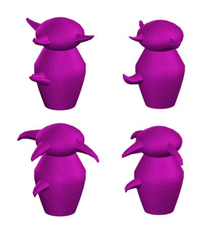
5 Empirical Study I: Greebles
As a first test-bed for GLAD using real data obtained from the Mechanical Turk, we posted pictures
of 100 “Greebles” [6], which are synthetically generated images that were originally created to study
human perceptual expertise. Greebles somewhat resemble human faces and have a “gender”: Males
have horn-like organs that point up, whereas for females the horns point down. See Figure 3 (left)
for examples. Each of the 100 Greeble images was labeled by 10 different human coders on the Turk
for gender (male/female). Four greebles of each gender (separate from the 100 labeled images) were
given as examples of each class. Shown at a resolution of 48x48 pixels, the task required careful
inspection of the images in order to label them correctly. The ground-truth gender values were all
known with certainty (since they are rendered objects) and thus provided a means of measuring the
accuracy of inferred image labels.
5Inferred Label Accuracy of Greeble Images
1
Accuracy (% correct)
0.95
0.9
GLAD
Majority Vote
0.85
2 3 4 5 6 7 8
Number of labels per image
Figure 3: Left: Examples of Greebles. The top two are “male” and the bottom two are “female.”
Right: Accuracy of the inferred labels, as a function of the number of labels M obtained for each
image, of the Greeble images using either GLAD or Majority Vote. Results were averaged over 100
experimental runs.
We studied the effect of varying the number of labels M obtained from different labelers for each
image, on the accuracy of the inferred Z. Hence, from the 10 labels total we obtained per Greeble
image, we randomly sampled 2 ≤ M ≤ 8 labels over all labelers during each experimental trial. On
each trial we compared the accuracy of labels Z as estimated by GLAD (using a threshold of 0.5
on p(Z)) to labels as estimated by the Majority Vote heuristic. For each value of M we averaged
performance for each method over 100 trials.
Results are shown in Figure 3 (right). For all values of M we tested, the labels as inferred by GLAD
are significantly higher than for Majority Vote (p < 0.01). This means that, in order to achieve the
same level of accuracy, fewer labels are needed. Moreover, the variance in accuracy was less for
GLAD than for Majority Vote for all M that were tested, suggesting that the quality of GLAD’s
outputs is more stable than of the heuristic method. Finally, notice how, for the even values of M ,
the Majority Vote accuracy decreases. This may stem from the lack of optimal decision rule under
Majority Vote when an equal number of labelers say an image is Male as who say it is Female.
GLAD, since it makes its decisions by also taking ability and difficulty into account, does not suffer
from this problem.
6 Empirical Study II: Duchenne Smiles
As a second experiment, we used the Mechanical Turk to label face images containing smiles as
either Duchenne or Non-Duchenne. A Duchenne smile (“enjoyment” smile) is distinguished from a
Non-Duchenne (“social” smile) through the activation of the Orbicularis Oculi muscle around the
eyes, which the former exhibits and the latter does not (see Figure 4 for examples). Distinguishing
the two kinds of smiles has applications in various domains including psychology experiments,
human-computer interaction, and marketing research. Reliable coding of Duchenne smiles is a
difficult task even for certified experts in the Facial Action Coding System.
We obtained Duchenne/Non-Duchenne labels for 160 images from 20 different Mechanical Turk
labelers; in total, there were 3572 labels. (Hence, labelers labeled each image a variable number of
times.) For ground truth, these images were also labeled by two certified experts in the Facial Action
Coding System. According to the expert labels, 58 out of 160 images contained Duchenne smiles.
Using the labels obtained from the Mechanical Turk, we inferred the image labels using either
GLAD or the Majority Vote heuristic, and then compared them to ground truth.
6Duchenne Smiles Non-Duchenne Smiles
Figure 4: Examples of Duchenne (left) and Non-Duchenne (right) smiles. The distinction lies in
the activation of Orbicularis Oculi muscle around the eyes, and is difficult to discriminate even for
experts.
Accuracy under Noise Accuracy under Adversarialness
0.8 1
0.78
0.9
0.76
0.8
Accuracy
Accuracy
0.74
0.7
0.72
0.6
0.7
0.68 0.5
GLAD GLAD
Majority Vote Majority Vote
0.66 0.4
0 1000 2000 3000 4000 5000 0 200 400 600 800
Num of Noisy Labels Num of Adversarial Labels
Figure 5: Accuracy (percent correct) of inferred Duchenne/Non-Duchenne labels using either
GLAD or Majority Vote under (left) noisy labelers or (right) adversarial labelers. As the number of
noise/adversarial labels increases, the performance of labels inferred using Majority Vote decreases.
GLAD, in contrast, is robust to these conditions.
Results: Using just the raw labels obtained from the Mechanical Turk, the labels inferred using
GLAD matched the ground-truth labels on 78.12% of the images, whereas labels inferred using
Majority Vote were only 71.88% accurate. Hence, GLAD resulted in about a 6% performance gain.
Simulated Noisy and Adversarial Labelers: We also simulated noisy and adversarial labeler con-
ditions. It is to be expected, for example, that in some cases labelers may just try to complete the task
in a minimum amount of time disregarding accuracy. In other cases labelers may misunderstand the
instructions, or may be adversarial, thus producing labels that tend to be opposite to the true labels.
Robustness to such noisy and adversarial labelers is important, especially as the popularity of Web-
based labeling tools increases, and the quality of labelers becomes more diverse. To investigate the
robustness of the proposed approaches we generated data from virtual “labelers” whose labels were
completely uninformative, i.e., uniformly random. We also added artificial “adversarial” labelers
whose labels tended to be the opposite of the true label for each image.
The number of noisy labels was varied from 0 to 5000 (in increments of 500), and the number of
adversarial labels was varied from 0 to 750 (in increments of 250). For each setting, label inference
accuracy was computed for both GLAD and the Majority Vote method. As shown in Figure 5, the
accuracy of GLAD-based label inference is much less affected from labeling noise than is Majority
Vote. When adversarial labels are introduced, GLAD automatically inferred that some labelers were
purposely giving the opposite label and automatically flipped their labels. The Majority Vote heuris-
tic, in contrast, has no mechanism to recover from this condition, and the accuracy falls steeply.
77 Related Work To our knowledge GLAD is the first model in the literature to simultaneously estimate the true label, item difficulty, and coder expertise in an unsupervised and efficient manner. Our work is related to the literature on standardized tests, particularly the Item Response Theory (IRT) community (e.g., Rasch [10], Birnbaum [3]). The GLAD model we propose in this paper can be seen as an unsupervised version of previous IRT models for the case in which the correct answers (i.e., labels) are unknown. Snow, et al [14] used a probabilistic model similar to Naive Bayes to show that by averaging mul- tiple naive labelers (
[3] A. Birnbaum. Some latent trait models and their use in inferring an examinee’s ability. Statistical theories
     of mental test scores, 1968.
 [4] N. Butko and J. Movellan. I-POMDP: An infomax model of eye movement. In Proceedings of the
     International Conference on Development and Learning, 2008.
 [5] A. Dawid and A. Skene. Maximum likelihood estimation of observer error-rates using the em algorithm.
     Applied Statistics, 28(1):20–28, 1979.
 [6] I. Gauthier and M. Tarr. Becoming a “greeble” expert: Exploring mechanisms for face recognition. Vision
     Research, 37(12), 1997.
 [7] V. Johnson. On bayesian analysis of multi-rater ordinal data: An application to automated essay grading.
     Journal of the American Statistical Association, 91:42–51, 1996.
 [8] G. Karabatsos and W. H. Batchelder. Markov chain estimation for test theory without an answer key.
     Psychometrika, 68(3):373–389, 2003.
 [9] Omron. OKAO vision brochure, July 2008.
[10] G. Rasch. Probabilistic Models for Some Intelligence and Attainment Tests. Denmark, 1960.
[11] S. Rogers, M. Girolami, and T. Polajnar. Semi-parametric analysis of multi-rater data. Statistics and
     Computing, 2009.
[12] V. Sheng, F. Provost, and P. Ipeirotis. Get another label? improving data quality and data mining using
     multiple noisy labelers. In Knowledge Discovery and Data Mining, 2008.
[13] P. Smyth, U. Fayyad, M. Burl, P. Perona, and P. Baldi. Inferring ground truth from subjective labelling of
     venus images. In Advances of Neural Information Processing Systems, 1994.
[14] R. Snow, B. O’Connor, D. Jurafsky, and A. Y. Ng. Cheap and fast - but is it good? evaluating non-expert
     annotations for natural language tasks. In Proceedings of the 2008 Conference on Empirical Methods on
     Natural Language Processing, 2008.
[15] S. Steinbach, V. Rabaud, and S. Belongie. Soylent grid: it’s made of people! In International Conference
     on Computer Vision, 2007.
[16] D. Turnbull, R. Liu, L. Barrington, and G. Lanckriet. A Game-based Approach for Collecting Semantic
     Annotations of Music. In 8th International Conference on Music Information Retrieval (ISMIR), 2007.
[17] L. von Ahn and L. Dabbish. Labeling Images with A Computer Game. In Proceedings of the SIGCHI
     conference on Human factors in computing systems, pages 319–326. ACM Press New York, NY, USA,
     2004.
[18] L. von Ahn, B. Maurer, C. McMillen, D. Abraham, and M. Blum. reCAPTCHA: Human-Based Character
     Recognition via Web Security Measures. Science, 321(5895):1465, 2008.

                                                       9
You can also read