Implementation of Deep Learning Using Convolutional Neural Network Algorithm for Classification Rose Flower
←
→
Page content transcription
If your browser does not render page correctly, please read the page content below

Journal of Physics: Conference Series

PAPER • OPEN ACCESS

Implementation of Deep Learning Using Convolutional Neural Network
Algorithm for Classification Rose Flower
To cite this article: Imania Ayu Anjani et al 2021 J. Phys.: Conf. Ser. 1842 012002

View the article online for updates and enhancements.

                                This content was downloaded from IP address 46.4.80.155 on 14/05/2021 at 21:38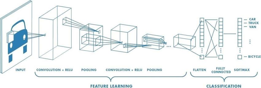
International Conference on Science Education and Technology (ICOSETH) 2020               IOP Publishing
Journal of Physics: Conference Series            1842 (2021) 012002 doi:10.1088/1742-6596/1842/1/012002

Implementation of Deep Learning Using Convolutional Neural
Network Algorithm for Classification Rose Flower

                     Imania Ayu Anjani1*, Yulinda Rizky Pratiwi2 and Norfa Bagas Nurhuda S.3
                     1,2,3
                             Bina Nusantara University, Jakarta, Indonesia

                     Email: 1* imania.anjani@binus.ac.id, 2 yulinda.pratiwi@binus.ac.id,
                     3
                         norfa.sukowati@binus.ac.id

                     Abstract. Flora in Indonesia has about 25% of the species of flowering plant species present in
                     the world. Roses are one type of flowering plants and are usually used as an ornamental plant
                     that has a thorny stem. Roses have more than 150 species. In Indonesia there are several flower
                     gardens that is larger than the others. One of the famous flower garden in Indonesia is located
                     on Malang city, East Java. The flower garden in Malang has several varieties of many roses and
                     has a large production of roses. To help the sales system of roses there, the researchers want to
                     create a program that can classify the type of roses in order to help simplify the system of
                     automatic sales of roses without through manual sorting. So that will accelerate the sale of roses
                     with an automated system. Ordinary people with limited botanical knowledge usually don’t
                     know how to classify the flowers just by looking at them. To classify the flowers properly, it is
                     important to provide enough information, and one of them is the name of it. Convolutional
                     Neural Network (CNN) is one method of deep learning that can be used for image classification
                     process. The CNN design is motivated by the discovery of the visual mechanism, the visual
                     cortex present in the brain. CNN has been widely used in many real-world applications, such as
                     Face Recognition, Image Classification and Recognition, and Object Detection, because this is
                     one of the most efficient method for extracting important features. In this research, the
                     classification accuracy value obtained from the test data is 96.33% using 2-dimension Red Green
                     Blue (RGB) input image, and the size of each image is 32 x 32 pixels that are trained with CNN
                     algorithm and the network structure of four convolution layers and four layers pooling supported
                     by dropout technique.

1. Introduction
Apart from being known as an agricultural country, Indonesia is also known as one of the countries that
has important role in the agricultural sector, because it has strategic location and large area. Based on
the data from the Ministry of Environment in 2013, Indonesia has an area of 1.3% of the earth's surface
and has high biodiversity (mega biodiversity), which is about 17% of all types of living things on this
earth. Indonesian flora is also part of Malesiana, because in the plant world Indonesia has about 25% of
the species of flowering plant species in the world [14].
   Convolutional Neural Network (CNN) is a deep learning method that can be used for image
classification process. CNN has been widely used in many applications in the real world, such asface
recognition, image recognition and recognition, and object detection because this method is one of the
most efficient methods for extracting features, and essential feature with less luminance task. The design

              Content from this work may be used under the terms of the Creative Commons Attribution 3.0 licence. Any further distribution
              of this work must maintain attribution to the author(s) and the title of the work, journal citation and DOI.
Published under licence by IOP Publishing Ltd                          1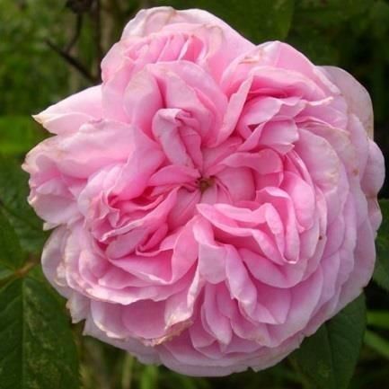
International Conference on Science Education and Technology (ICOSETH) 2020               IOP Publishing
Journal of Physics: Conference Series            1842 (2021) 012002 doi:10.1088/1742-6596/1842/1/012002

of the Convolutional Neural Network was motivated by the discovery of a visual mechanism, namely
the visual cortex in the brain.
    Flower classification has a wide range of applications, as it helps in finding the name of flowers in
floriculture, automating the floriculture system and more. Based on the above background, this study
will implement the implementation of the deep learning method using CNN to classify roses which aims
to help introduce several types so that people who do not know the types of roses can find out what types
of roses are in the image and the program created can be applied to the flower sales system automatically
without asking the seller what the name of the flower is. This study focuses on how to classify the image
of roses into several types.

2. Theoretical Basis

2.1. Roses
   Roses are one of the cut flowers that are most in demand by the community, where they are often
used as decorative flowers at formal events such as seminars, workshops or non-formal events such as
weddings and traditional events. The general characteristics of a rose flower are that it grows like a
shrub that has a height of approximately 2 meters, has an upright round stems with spiny greenish green,
leaves about 5-10 cm long and 1.5-2.5 cm wide, the flowers smell nice and taproot.

2.1.1. Burgundy Red Roses
    This Burgundy rose is a red rose which is very popular in the world. This flower has a flower size
between 8-10 cm and can bloom more than once a season. This flower is included in the type of Hybrid
rose. Burgund flowers have a plant height that ranges from 40-45cm.Formatting author names The list
of authors should be indented 25 mm to match the abstract. The style for the names is initials then
surname, with a comma after all but the last two names, which are separated by ‘and’. Initials should
not have full stops—for example A J Smith and not A. J. Smith. First names in full may be used if
desired. If an author has additional information to appear as a footnote, such as a permanent address or
to indicate that they are the corresponding author, the footnote should be entered after the surname.

                               Figure 1. Burgundy Rose (Route10Garden, 2018)

2.1.2. Osiana Roses
   This Osiana flower was a popular cut flower from the early 1980s. It is known as a cut flower that
grows outdoors and originates in Germany and is known throughout the world. Osiana flowers have a
very elegant face, are large and have a fruity fragrance. The size of this flower ranges from 8-10cm. The
color of this flower is creamy white and has a plant height of 100-130cm.

                                                    2
International Conference on Science Education and Technology (ICOSETH) 2020               IOP Publishing
Journal of Physics: Conference Series            1842 (2021) 012002 doi:10.1088/1742-6596/1842/1/012002

                                    Figure 2 Osiana Rose (Rosto4ek, 2018)

2.1.3. Damascus Roses
    Considered to be one of the oldest roses from Europe, Damascus Rose is also known as Rose of
Catile or Damascus Rose. These flowers make a very enchanting choice for a bouquet or bouquet
because they have a very strong fragrance. Today, Damascus roses are widely grown throughout Europe.
Some of the benefits of this flower are that the petals can be used for making perfume, as a food spice
and are widely used in the cosmetic industry. This Damascus rose can be found in the bush that is quite
tall, has a soft texture and is quite large. Usually these flowers are pastel pink and some have a strong
sweet aroma and have a flower petal length of 3-4 inches.

                                 Figure 3. Damascus Roses (Gramunion, 2018)

2.2. Imagery
    Image is a representation or description, imitation or similarity of an object. Literally, an image is an
image that has a two-dimensional (two-dimensional) plane size. From a mathematical point of view,
image is a continuous function of light intensity in a two-dimensional plane. The image comes from the
reflection of light that illuminates several objects, then this light reflection is captured by optical devices
such as the eye, the camera so that the image of the object is formed as an image that can be recorded.
In another sense, the image is the output of a data recording system, one of which is optical in the form
of photos, analog in nature, which is in the form of video signals such as images on a television monitor
screen and can also be digital which can be stored on a storage medium [26].
    Digital Image is an image arranged in the form of a grid, where each box formed is called a pixel and
has a two-dimensional function f (x, y) with coordinates (x, y). The x-axis represents rows and the y-
axis represents columns. Each pixel has a value that indicates the color intensity of that pixel. Figure.

2.2.1. below shows the coordinates of the digital image.
    Digital images are usually written with a matrix of size N x M, where N is the column / height while
M is the row / width. There are two parameters that are owned by pixels, namely coordinates and color
intensity. The value contained in the coordinates (x, y) is the amount of color intensity of the pixels in

                                                       3
International Conference on Science Education and Technology (ICOSETH) 2020 IOP Publishing
Journal of Physics: Conference Series 1842 (2021) 012002 doi:10.1088/1742-6596/1842/1/012002
that point. Several formats of digital images are BMP, PNG, JPG, GIF and others (Kusumanto and
Tompunu, 2011).
Figure 4. Koordinat Citra Digital (Sutoyo dkk, 2009)
2.2.2. Convulotional Neural Network
“Convolutional Neural Network (CNN) is a development of Multilayer Perceptron (MLP) which is
designed to process two-dimensional data. CNN is included in the type of Deep Neural Network because
of its high network depth and is widely applied to image data. In the case of image classification, MLP
is not suitable for use because it does not store spatial information from image data and considers each
pixel to be an independent feature, resulting in unfavorable results” [2].
The convolutional layer in CNN performs functions that are performed by cells in the visual cortex.
In general, the convolutional layer will detect features in the form of edges on the image, then the
subsampling layer will reduce the dimensions of the features obtained from the convolutional layer, and
finally forward it to the output node through the forward propagation process, and the prediction of the
data class is finally determined by the method. Softmax on the dense layer or fully connected layer [12].
Figure 5. Convolutional Neural Network Architecture (Douglas, 2018)
2.3. Back Propagation Algorithm
The Back-Propagation Algorithm is a popular algorithm used in the training phase of an artificial
neural network. According to the Fundmental of Neural Networks book, basically this algorithm is
divided into three important stages, namely the forward propagation section, then the back- propagation
error section, and finally the weight adjustment section or the weight adjustment phase [3]. The weight
referred to in this algorithm is the value contained in the link between neurons in the artificial neural
network structure.
4International Conference on Science Education and Technology (ICOSETH) 2020 IOP Publishing
Journal of Physics: Conference Series 1842 (2021) 012002 doi:10.1088/1742-6596/1842/1/012002
In the forward propagation phase, the input layer x will continue the input through the connection v,
then enter the hidden layer z, to calculate the input value in the hidden layer, the equation below can be
used [3] where i is the index of the input neuron, j is index of hidden neurons and n is the total number
of input neurons.
In this layer the activation value will be calculated with a function of each neuron which will then be
forwarded to each neuron in the output layer with equation below :
On the Back-propagation Net, after the criteria for stopping are reached, the weights obtained will
be stored and will then be used as weights in the testing phase. This testing phase is to perform the
forward propagation phase using input that has never been trained, and utilizing the weights obtained
from the training phase earlier.
3. Research Methodology
3.1. Population and Sample
The population in this study is in the form of images or objects of roses. There are 3 types of roses
used, namely burgundy roses, osiana roses and damascus roses. As for the sample used in this study
amounted to 150 images where each type or class of each 50 images of roses.
The text of your paper should be formatted as follows:
3.1.1. Variables and Variable Operational Definitions
The variables used in this study are shown in Table 4.1 regarding the explanation and operational
definition of the research which is an explanation of each variable.
Table 1. Variable Operational Definitions
No Variable Code Variable Operational Definitions
1 Burgundy Roses ‘ht(number).jpg Image of burgundy roses
2 Osiana Roses ‘or(number).jpg Image of osiana roses
3 Damascus Roses ‘dr(number).jpg Image of damascus roses
3.1.2. Types and Sources of Data
The type of data used in this study is secondary data. The data is obtained by crawling the image of
puppet characters on the Google search engine using Fatkun Image Downloader. This software is an
additional feature of Google Chrome.
3.1.3. Data Analysis Method
Some of the data analysis used in this study are as follows:
1) Image histogram, which is used to view the representation of color distribution in an image.
2) Deep Learning method, namely Convolutional Neural Network, is used to classify images or
images.
3) The number of convolutional layers used in this study is 4 layers and the activation function used
in this study is ReLU.
4) Researchers will conduct several testing scenarios to be able to choose the best model. The
predetermined test scenarios are the comparison of the input size, the dropout size on the last layer,
the number of neurons in the last layer and the training and testing data partitions.
5) In selecting the best model for object (image) classification in the Convolutional Neural Network
algorithm, the researcher will choose the best model in terms of accuracy and loss values from the
comparison of the test scenarios in point 4 above. The best model chosen is the one with the highest
5International Conference on Science Education and Technology (ICOSETH) 2020 IOP Publishing
Journal of Physics: Conference Series 1842 (2021) 012002 doi:10.1088/1742-6596/1842/1/012002
accuracy value and the smallest loss value.
4. Result of Analysis
4.1. Image Histogram
One of the formats that can be used to display image data is image data with three degrees of color,
namely red (red), green (green) and blue (blue) or often referred to as RGB. In this study, the image of
the rose to be used is a color image, so there is no need to change the downloaded image. The following
is an example of a representation of a rose image obtained using Rstudio software. The use of sections
to divide the text of the paper is optional and left as a decision for the author. Where the author wishes
to divide the paper into sections the formatting shown in table 2 should be used.
Figure 6. Damascus Roses (HobbyKafe, 2015)
The rose image above has a lot of information contained, including pixel size, image channel and
image histogram which can represent the basic formation of the image above. The process of image
manipulation can be done with the help of R. software.
Image
colorMode : Color
storage.mode : double
dim
: 500 500 3
frames.total : 3
frames.render: 1
imageData(object)[1:5,1:6,1]
[,1] [,2] [,3] [,4] [,5] [,6]
[1,] 0.3764706 0.3725490 0.3647059 0.3529412 0.3372549 0.3176471
[2,] 0.3647059 0.3607843 0.3529412 0.3411765 0.3254902 0.3098039
[3,] 0.3529412 0.3490196 0.3411765 0.3294118 0.31764710.3019608
[4,] 0.3450980 0.3411765 0.3333333 0.3254902 0.3137255 0.3019608
[5,] 0.3490196 0.3450980 0.3372549 0.3294118 0.3215686 0.3137255
Figure 7. Image Information
The image above includes an RGB color image marked with the meaning of color on the colorMode
line. The dimension size of the image above is 500x500 pixels and has an RGB channel of The value or
number in the matrix form above describes the brightness level of a color at each pixel of the rose image
above, but the value that can be displayed is only up to the fifth line. and the sixth column only because
of limitations in displaying output in RStudio.
The representation of the RGB distribution of the Damascus rose image is shown in the following
figure. The resulting histogram contains a numeric value of 750000 pixels. This value is obtained from
the multiplication of the dimensions of the image size, namely 500 x 500 x 3, which indicates the number
of elements or parts that make up the image.
6International Conference on Science Education and Technology (ICOSETH) 2020 IOP Publishing
Journal of Physics: Conference Series 1842 (2021) 012002 doi:10.1088/1742-6596/1842/1/012002
Figure 8. Image Histogram
4.2. Effect of Input Size Scenarios
The image size used can affect the detail of the image on the flower. In general, if you use a larger
input image size, the accuracy value of the test data will be higher. In this study, the size of the input
image measuring 32 x 32 pixels will be compared with the input image measuring 64 x 64. The results
of the input image size comparison scenario are shown in table 4.2 below.
Table 2. Input Size Determination Scenarios
Input Size Scenarios Data Training Accuracy Data Testing Accuracy
32 x 32 100% 96,66 %
64 x 64 90,83% 70 %
The experimental results shown in the table above can be seen that data with an input image size of
32 x 32 pixels has a higher accuracy than data with an input image size of 64 x 64 pixels, both for testing
and training data. The input size that will be used for the next analysis process is 32 x 32 pixels. Then
the dropout value will be compared which will be selected the best for the next analysis process.
4.3. The Effect of the Dropout Scenario on the Last Layer
The overfitting of the model can be overcome by implementing a regularization method such as
dropout. The dropout method was used in a study in 2014, this study showed a decrease in the error
graph of the two same network structures when subjected to the dropout method (Srivastava, et al.,
2014). The use of dropout probability can affect the performance of CNN. Regarding the dropout
method, in applying this method there is a probability that must be determined. This probability
represents the number of units that will dropout a layer. There is no research that can determine how
many probabilities should be used, but the probability values that can be used range from 0 to 1. In this
study, the researcher wants to compare several dropout probability values. The results of the comparison
scenario using the dropout value are shown in table 4.3.1 below.
Table 3. Dropout Determination Scenarios
Last Dropout Layer Scenarios Accuracy Data Training : Loss Data Training : Data
Data Testing Testing
0,1 % 72,5% : 73,33% 0,634 : 0,684
0,01% 100% : 96,66% 0,0194 : 0,304
0,001% 100% : 96,66% 0,0011 : 0,0307
7International Conference on Science Education and Technology (ICOSETH) 2020 IOP Publishing
Journal of Physics: Conference Series 1842 (2021) 012002 doi:10.1088/1742-6596/1842/1/012002
Based on the comparison table above, the application of a dropout with a probability of 0.001% has
the highest accuracy value and the lowest loss value when compared to the dropout probability values
of 0.1% and 0.01%. From this table it can also be seen that the use of the dropout probability value of
0.01% and 0.001% has the same accuracy value in the test data and training data. What distinguishes
between the two is the result of the loss value on the test data and training data. The dropout probability
value of 0.001% has a loss value that is smaller than the dropout value of 0.01%. The best model of this
scenario is to use a dropout probability of 0.001%. The dropout value in the last layer that will be used
for the next analysis process is 0.001%. Then the number of neurons in the last layer will be compared
which will be selected the best for the next analysis process.
Table 4 Scenario Determination of Neurons Number
Last Dropout Layer Scenarios Accuracy Data Training : Data Loss Data Training : Data
Testing Testing
125 100% : 96,66% 0,0011 : 0,0307
250 100% : 96,66% 0,0005 : 0,105
The number of neurons that gave the smallest loss value was 125. The number of neurons in this
study did not affect the accuracy of the model, but it did affect the loss value in the training and testing
data. The best model of this scenario is to use the number of neurons of 125. The number of neuron
layers in the last layer that will be used for the next analysis process is 125. Then the scenario of sharing
(partitioning) training and testing data will be selected which is the best.
Table 5. Scenario of Total Data Training and Testing
Data Training : Data Count of Data Training : Data Testing Loss Value
Testing Scenarios Data Testing Accuracy
60% : 40% 90 : 60 96,66 % 0,0909
70% : 30% 105 : 45 95,55% 0,1629
80% : 20% 120 : 30 96,66 % 0,0307
The best result of this scenario is to use a data training and testing scenario with a ratio of 80%: 20%.
When compared with other scenarios, the accuracy of the 80%: 20% data partition has the highest
accuracy value and the lowest loss value of the 70%: 30% data partition and 60%: 40%. This happens
because the learning process is carried out with more training data, the system will also learn more than
other scenarios.
5. The Best Scenario
The best model chosen is the model that has the highest accuracy value for training data and testing
data from all scenario testing. The test in the first scenario is to compare the size of the image input
between 32 x 32 pixels and 64 x 64 pixels. In this first scenario testing, the selected model is the image
input size of 32x32 pixels because it has a higher accuracy value on the test data, namely 96.66% than
the image input size of 64x64 pixels, namely 70%. The test in the second scenario is to compare the
dropout value in the last layer, which is between 0.1%, 0.01% and 0.001%.
The application of a dropout with a probability of 0.001% has the highest accuracy value and the
lowest loss value when compared to the dropout probability value of 0.1% and 0.01%. From this table
it can also be seen that the use of the dropout probability value of 0.01% and 0.001% has the same
accuracy value in the test data and training data. What distinguishes between the two is the result of the
loss value on the test data and training data. The dropout probability value of 0.001% has a loss value
that is smaller than the dropout value of 0.01%.
8International Conference on Science Education and Technology (ICOSETH) 2020 IOP Publishing
Journal of Physics: Conference Series 1842 (2021) 012002 doi:10.1088/1742-6596/1842/1/012002
The best model of this scenario is to use a dropout probability of 0.001%. Testing in the third scenario
is to compare the number of neurons in the last layer, which is between 125 and 250. The number of
neurons giving the smallest loss value is 125. The number of neurons in this study does not affect the
accuracy of the model, but affects the loss value in training and testing data. The best model of this
scenario is to use the number of neurons of 125. Testing in the last scenario is to compare the distribution
of training data and testing data, namely between 60%: 40%, 70%: 30% and 80%: 20%.
The best result of this scenario is to use a data training and testing scenario with a ratio of 80%: 20%.
When compared with other scenarios, the accuracy of the 80%: 20% data partition has the highest
accuracy value and the lowest loss value of the 70%: 30% data partition and 60%: 40%. The best model
chosen is a network using 4 convolution layers, 2 pooling layers, 3x3 kernel size, a softmax layer, a
fully connected layer, 32 filters on convolution layers 1 and 2, 64 filters on convolution layers 1 and 2.
, the dropout value after the first pooling layer is 0.1%, the dropout value after the second pooling layer
is 0.01%, the input size is 32 x 32 pixels, the dropout value on the last layer is 0.001%, the number of
neurons in the last layer is 250 and the distribution training and testing data of 80%: 20%.
Table 6. Accuracy Results on Training and Testing Data
Data Count Loss Accuracy
Training 120 0,001126901 100%
Testing 30 0,03076569 96,66%
The plot of the performance results from the loss and accuracy values generated from the model that
was formed can be shown in Figure 9 below.
Figure 9. Plots of Acurracy and Loss Value Result
Based on table 5.1, it can be seen that the resulting loss value in the training data is 0.001126901.
When compared with the loss value in the testing data, the loss value in the training data is smaller so
that this value can be said to be quite low and good from the model obtained. This is supported by the
high accuracy value for each data. The training data has an accuracy value of 100% and 96.66% on the
testing data. The resulting model can be said to be able to classify well because it has a low loss value
and high accuracy value.
The results of the classification on the training data can be shown in the confusion matrix table below.
9International Conference on Science Education and Technology (ICOSETH) 2020 IOP Publishing
Journal of Physics: Conference Series 1842 (2021) 012002 doi:10.1088/1742-6596/1842/1/012002
Table 7. Classification Results on Training Data
Burgundy Osiana Damascus
Burgundy 40 0 0
Osiana 0 40 0
Damascus 0 0 40
From the table above, it can be seen that in the training data all images are classified appropriately
by the formed model and there is no error at all in the classification process. This can also be seen from
the accuracy value generated in the training data, which is 100%. The classification results of the testing
data can be seen in the following table 7 confusion matrix.
Table 8 Classification Results on Training Data
Burgundy Osiana Damascus
Burgundy 10 1 0
Osiana 0 9 0
Damascus 0 0 10
The classification results on the testing data as shown in table 4 can provide an explanation that not
all images are classified correctly into their class. This can be seen from the classification results of the
Osiana rose. In the table, out of 10 images of the Osiana rose, there are 1 image misclassification.
6. Conclusion
The best model for classifying roses flower is obtained from 32 x 32 pixel images, with the combination
of 4 convolution layers, 2 pooling layers, 3x3 kernel size, one softmax layer, and a fully connected layer.
This model reached 96.33% in accuracy with RGB images. But the accuracy decreases with 64 x 64
pixel images. Further research should be focused on increasing the accuracy with 64 x 64 pixel images,
as this research can only get roughly 70% in accuracy.
References
[1] Dewa, C. K., Fadhilah, A. L., & Afiahayati. (2018). Convolutional Neural Networks for
Handwritten Javanese Character Recognition. IJCCS (Indonesian Journal of Computing and
Cybernetics Systems), 93-94.
[2] E.P, I. W., Wijaya, A. Y., & Soelaiman, R. (2016). Klasifikasi Citra Menggunakan Convolutional
Neural Network (Cnn) pada Caltech 101. JURNAL TEKNIK ITS, A65-A69.
[3] Fausett, L., (1994). Fundamentals of Neural Networks: Architectures, Algorithms, and
Applications. Prentice-Hall international editions. Upper Saddle River, New Jersey: Prentice-
Hall.
[4] Fawcett, T., (2006). An introduction to ROC analysis. Pattern Recognition Letters 27, pp. 861-
874.
[5] Fresh, F. (2017). Types of Roses: A Visual Compendium. Dipetik April 22, 2018, dari FTD.COM:
https://www.ftd.com/blog/share/types-of-roses
[6] Google Image Search. (2018). Osiana, Burgund, Damask. Diakses tanggal 21 Juni 2018 pukul
16.00 dari Google Image Search : images.google.com
[7] Gramunion. (2018). Champagne Blossom. Diakses tanggal 20 Juni 2018 pukul 19.20 dari
Gramunion :
HYPERLINK"http://www.gramunion.com/champagneblossom.tumblr.com?page=9"
http://www.gramunion.com/champagneblossom.tumblr.com?page=9
[8] Gurnani, A., Mavani, V., Gajjar, V., & Khandhediya, Y. (2017). Flower Categorization using
Deep Convolutional Neural Networks. ARXIV (Computer Vision and Pattern Recognition), -.
[9] Hanum, C. (2008). Teknik Budidaya Tanaman. Direktorat Pembinaan Sekolah Menengah
10International Conference on Science Education and Technology (ICOSETH) 2020 IOP Publishing
Journal of Physics: Conference Series 1842 (2021) 012002 doi:10.1088/1742-6596/1842/1/012002
Kejuruan. Direktorat Jenderal Manajemen Pendidikan Dasar dan Menengah, Departemen
Pendidikan Nasional.
[10] Hao, D. C., Gu, X.-J., & Xiao, P. G. (2015). Potentilla and Rubus medicinal plants: potential non-
Camellia tea resources. Medicinal Plants, 373-430.
[11] Heaton, J., (2015). AIFH, Volume 3: Deep Learning and Neural Networks. Washington DC:
Heaton Research, Inc..
[12] Hijazi, S., Kumar, R., & Rowen, C. (2015). Using convolutional neural networks for image
recognition. Cadence Design Systems Inc.: San Jose, CA, USA.
[13] HobbyKafe. (2015). Rose. Diakses tanggal 20 Juni 2018 pukul 19.50 dari Gramunion :
https://hobbykafe.com/forum/viewtopic.php?t=1240&start=3285
[14] Kusmana, C., & Hikmat, A. (2015). Keanekaragaman hayati flora di Indonesia. Jurnal
Pengelolaan Sumberdaya Alam dan Lingkungan (Journal of Natural Resources and
Environmental Management),vol. 5(no.2), hal.187.
[15] LeCun, Y., Bengio, Y., & Hinton, G. (2015, Mei 27). Deep Learning. Retrieved from Nature
International Journal of Science: doi:10.1038/nature14539
[16] Mahanta, J. (2017). Introduction to Neural Networks, Advantages and Applications. Diakses
tanggal 5 April 2018 pukul 19.30 dari Towards Data Science:
https://towardsdatascience.com/introduction-to- neural-networks-advantages-and-
applications-96851bd1a207
[17] Marwoto, Budi. (2017). Pasar Internasional Tanaman Hias Terbuka. Diakses tanggal 3 April
2018 pukul 20.48 dari https://www.suaramerdeka.com/news/baca/15810/pasar-internasional-
tanaman-hias- terbuka-lebar
[18] Maulida, Juwita.D. (2017). Penerapan Klasifikasi Algoritma Naive Bayes, Multilayer
Perceptron, Decision Tree J48 Dan Reptree. Skripsi. Fakultas Matematika dan Ilmu
Pengetahuan Alam. Universitas Islam Indonesia : Yogyakarta.
[19] Phetphoung, W., Kittimeteeworakul, N., & Waranusast, R. (2014). Automatic Sushi
Classification from Images using Color Histograms and Shape Properties. Student Project
Conference (ICT, IEEE), -.
[20] Priyanta, Ida.B.G.B. (2017). Pengenalan Topeng Bali Menggunakan Algoritma Convolutional
Neural Network. Tesis. Fakultas Matematika dan Ilmu Pengetahuan Alam. Universitas Gadjah
Mada : Yogyakarta.
[21] Rosto4ek. (2018). Osiana. Diakses tanggal 20 Juni 2018 pukul 19.10 dari Rosto4ek:
HYPERLINK "http://rosto4ek.com/osiana" http://rosto4ek.com/osiana
[22] Route10GardenCenter. (2018). Roses. Diakses tanggal 20 Juni 2018 pukul 19.00 dari Route10
Garden Center : HYPERLINK
"http://www.route10gardencenter.com/roses-1/"
http://www.route10gardencenter.com/roses-1/ .
[23] Shafira, Tiara. (2018). Implementasi Convolutional Neural Networks Untuk Klasifikasi Citra
Tomat Menggunakan Keras. Skripsi. Fakultas Matematika dan Ilmu Pengetahuan Alam.
Universitas Islam Indonesia : Yogyakarta.
[24] Sun, Julie. (2018). AI Model Training Pltaform. Diakses tanggal 21 Juni 2018 pukul 19.40 dari
JulieSun.com : HYPERLINK "http://www.juliesun.com/img/portfolio/UX-CaseStudy-AI-
JulieSun- preview.pdf" http://www.juliesun.com/img/portfolio/UX-CaseStudy-AI-JulieSun-
preview.pdf
[25] Srivastava, Nitish., Hinton, Geoffrey., Krizhevskey, Alex., Sutskever, Ilya dan Salakhutdinov,
Ruslan. (2014). Dropout: A Simple Way to Prevent Neural Networks from Overfitting. Journal
of Machine Learning Research 15, pp. 1929-1958.
[26] Sutoyo, T., Mulyanto, Edy., Suhartono, Vincent., Nurhayati, Oki Dwi dan Wijanarto. (2009).
Teori Pengolahan Citra Digital. Yogyakarta: Penerbit Andi.
11You can also read