Automatic Cephalometric Landmark Detection on X-ray Images Using a Deep-Learning Method - MDPI
←
→
Page content transcription
If your browser does not render page correctly, please read the page content below
applied
           sciences
Article
Automatic Cephalometric Landmark Detection on
X-ray Images Using a Deep-Learning Method
Yu Song 1,† , Xu Qiao 2,† , Yutaro Iwamoto 1 and Yen-wei Chen 1, *
 1    Graduate School of Information Science and Eng., Ritsumeikan University, Shiga 603-8577, Japan;
      gr0398ep@ed.ritsumei.ac.jp (Y.S.); yiwamoto@fc.ritsumei.ac.jp (Y.I.)
 2    Department of Biomedical Engineering, Shandong University, Shandong 250100, China; qiaoxu@sdu.edu.cn
 *    Correspondence: chen@is.ritsumei.ac.jp
 †    These authors contributed equally to this work.

 Received: 30 November 2019; Accepted: 6 February 2020; Published: 7 April 2020

 Abstract: Accurate automatic quantitative cephalometry are essential for orthodontics. However,
 manual labeling of cephalometric landmarks is tedious and subjective, which also must be performed
 by professional doctors. In recent years, deep learning has gained attention for its success in
 computer vision field. It has achieved large progress in resolving problems like image classification
 or image segmentation. In this paper, we propose a two-step method which can automatically
 detect cephalometric landmarks on skeletal X-ray images. First, we roughly extract a region of
 interest (ROI) patch for each landmark by registering the testing image to training images, which
 have annotated landmarks. Then, we utilize pre-trained networks with a backbone of ResNet50,
 which is a state-of-the-art convolutional neural network, to detect each landmark in each ROI patch.
 The network directly outputs the coordinates of the landmarks. We evaluate our method on two
 datasets: ISBI 2015 Grand Challenge in Dental X-ray Image Analysis and our own dataset provided by
 Shandong University. The experiments demonstrate that the proposed method can achieve satisfying
 results on both SDR (Successful Detection Rate) and SCR (Successful Classification Rate). However,
 the computational time issue remains to be improved in the future.

 Keywords: cephalometric landmark; X-ray; deep learning; ResNet; registration

1. Introduction
     Cephalometric analysis is performed on skeletal X-ray images. This is necessary for doctors to
make orthodontic diagnoses [1–3]. In cephalometric analysis, the first step is to detect landmarks
in X-ray images. Experienced doctors are needed to identify the locations of the landmarks.
Measurements of the angles and distances between these landmarks greatly assist diagnosis and
treatment plans. The work is time-consuming and tedious, and the problem of intra-observer variability
arises since different doctors may differ considerably in their identification of landmarks [4].
     Under these circumstances, computer-aided detection, which can automatically identify
landmarks objectively, is highly desirable. Studies on anatomical landmark detection have a long
history. In 2014 and 2015, International Symposium on Biomedical Imaging (ISBI) launched challenges
on cephalometry landmark detection [5,6], and several state-of-the-art methods were proposed.
In 2015’s challenge, Lindner and Cootes’s method based on random-forest achieved the highest
results, with a successful detection rate of 74.84% for a 2-mm precision range [7] (since landmark
location cannot be exactly same with manual annotation, Errors within a certain range are acceptable.
Usually, medically acceptable range is 2 mm). Ibragimov et al. achieved the second highest result
in 2015’s challenge, with a successful detection accuracy of 71.7% within a 2-mm range [8]. They
applied Haar-like feature extraction with a random-forest regression, then making refinements with

Appl. Sci. 2020, 10, 2547; doi:10.3390/app10072547                            www.mdpi.com/journal/applsci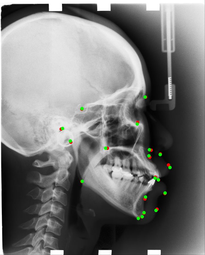
Appl. Sci. 2020, 10, 2547                                                                            2 of 16

a global-context shape model. In 2017, Ibragimov et al. added a convolutional neural network for
binary classification to their conventional method. They surpass the result of Lindner’s a little bit, with
around 75.3% prediction accuracy within a 2-mm range [9]. In 2017, Hansang Lee et al. proposed a
deep learning based method which achieved not bad results but in a small resized image. He trained
two networks to regress the landmark’s x and y coordinate directly [10]. In 2019, Jiahong Qian et al.
proposed a new architecture called CephaNet which improves the architecture of Faster R-CNN [11,12].
Its accuracy is nearly 6% higher than other conventional methods.
      Despite the variety of techniques available, automatic cephalometric landmark detection remains
insufficient due to its limited accuracy. In recent years, deep learning has gained attention for its
success in computer vision field. For example, convolutional neural network models are widely used in
problems like landmark detection [13,14], image classification [15–17] and image segmentation [18,19].
Trained models’ performances surpass that of human beings in many applications. Since direct
regression of several landmarks is a highly non-linear mapping, which is difficult to learn [20–23]. In
our method, we only try to detect one key point in one patch image. We learn a non-linear mapping
function for only one key point. Each key point has its corresponding non-linear mapping function. So
we can achieve more accurate detection of key point than other methods.
      In this paper, we propose a two-step method for the automatic detection of cephalometric
landmarks. First, we get the coarse landmark location by registering the test image to a most similar
image in the training set. Based on the registration result, we extract an ROI patch centered at the
coarse landmark location. Then, by using our pre-trained network with the backbone of ResNet50,
which is a state-of-the-art convolutional neural network, we detect the landmarks in the extracted ROI
patches to make refinements. The experiments demonstrate that our two-step method can achieve
satisfying results compared with other state-of-the-art methods.
      The remainder of this paper is organized as follows: We describe the study materials in Section 2.
In Section 3, we explain the proposed method in detail. Then, in Section 4, we describe the experiments
and discuss the results. Lastly, we present the conclusion in Section 5.

2. Materials

2.1. Training Dataset
      The training dataset is the 2015 ISBI Grand Challenge training dataset [6]. It contains 150 images,
each of which is 1935 × 2400 pixels in TIFF format. Each pixel’s size is 0.1 × 0.1 mm. The images
were labeled by two experienced doctors. We use the average coordinate value of the two doctors as
ground-truth for training.
      We aim to detect 19 landmarks for each X-ray image, as presented in Figure 1, which are as follows:
sella turcica, nasion, orbitale, porion, subspinale, supramentale, pogonion, menton, gnathion, gonion,
lower incisal incision, upper incisal incision, upper lip, lower lip, subnasale, soft tissue pogonion,
posterior nasal spine, anterior nasal spine, and articulate.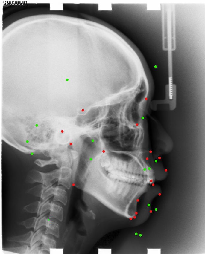
Appl. Sci. 2020, 10, 2547                                                                             3 of 16

                            Figure 1. All 19 landmarks on x-ray images which we aim to detect.

Data Augmentation
     The size of an X-ray image is 1935 × 2400 pixels. The scale is too huge to input the whole image
into a CNN to detect the locations of all 19 landmarks simultaneously. Therefore, we decide to detect
landmarks in small patches. In each patch, only one landmark will be detected. We train one model
for one landmark. Overall, we have 19 landmarks since there are 19 landmarks to be detected. These
models have the same architecture but different weights, as presented in Figure 2.
     In order to do data augmentation, we select 400 patches randomly for each landmark in one
training image. Each patch is 512 × 512 pixels. The landmark could be everywhere in the patch. Its
coordinate (x,y) in the ROI patch is used as teaching signal (ground truth) for training. Then, we resize
them into 256 × 256 patches, as presented in Figure 3. This means we will have 60,000 (400 × 150)
images to train one model for landmark i (i = 1, 2, ... 19).

                  Figure 2. We train 19 networks with same architecture but with different weights.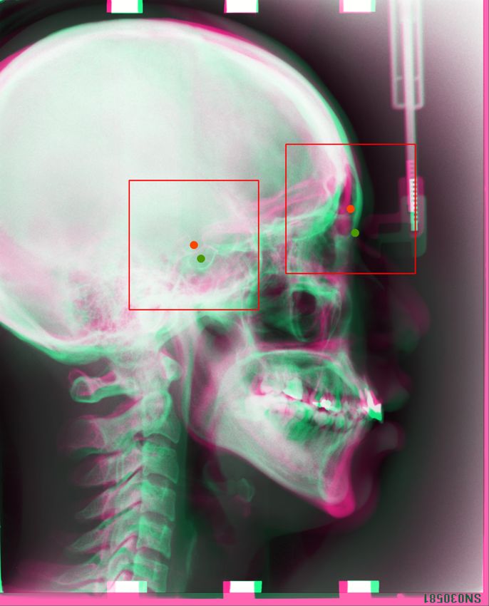
Appl. Sci. 2020, 10, 2547                                                                                  4 of 16

        (a) Example of our training image,          (b) The cropped 512 × 512 patch           (c) The resized 256
        the red boxes are cropped training                                                    × 256 patch
        images.
      Figure 3. The way we crop ROI patches for each landmark: the blue dot is a target landmark, the red
      boxes are extracted 512 × 512 ROI patches. We can see the landmark is included in all the ROI patches.
      We randomly extract 400 patches for one landmark in one x-ray image for training. Then we resize the
      ROI patches into 256 × 256 to make predictions.

2.2. Test Dataset
     We have two test datasets. Both datasets are tested through the models, which are trained with
the ISBI training dataset.

2.2.1. International Symposium on Biomedical Imaging (ISBI) Test Dataset
     The first test dataset from the ISBI Grand Challenge includes two parts: Test Dataset 1 with
150 test images and test dataset 2 with 100 images. The ISBI test images are collected with the same
machine as the training data, and each image is 1935 × 2400 in TIFF format.

2.2.2. Our Dataset
     Our own dataset is provided by Shandong University, China. In contrast to the ISBI dataset, the
data are taken with different machines. There are 100 images, each of which is 1804 × 2136 in JPEG
format.
     Also, the landmarks labeled by the doctors are not exactly the same as those in the ISBI dataset (13
of them are same). We used labels for sella turcica, nasion, orbitale, porion, subspinale, supramentale,
pogonion, menton, gnathion, gonion, lower incisal incision, upper incisal incision, and anterior nasal
spine. Other landmarks were not labeled by the doctors.

2.2.3. Region Of Interest (ROI)
     Extracted ROI patches are used as input images in our corresponding models. The method of
extraction is described in detail in Section 3.

3. Proposed Method

3.1. Overview
    The method is a two-step method: ROI extraction and Landmark detection. For ROI extraction,
we crop patches by registering the test image to training images, which have annotated landmarks.
Then, we use pre-trained CNN models with the backbone of ResNet50, which is a state-of-the-art
CNN, to detect the landmarks in the extracted ROI patches. The procedure is presented in Figure 4.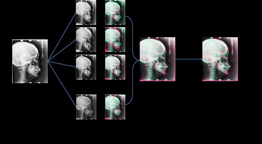
Appl. Sci. 2020, 10, 2547                                                                            5 of 16

                              Figure 4. The overview of our two-step method.

3.2. Automatic ROI Extraction
      Because of the limitation of the input image size, we aim to extract small ROI patches automatically.
That is, we extract ROI patches that include landmark i (i = 1, 2, 3. . . 19). To extract the ROI
automatically, we use registration to locate a coarse location of the landmark. Next, we extract
the ROI patch centered on the coarse location. Thus, the landmark location we aim to detect will be
included in the ROI patch.
      In this process, the test image is registered to training images, which have annotated landmarks.
We consider the test images as moving images and the training images as reference images. The type
of transform that we used is translation transform. The optimizer is gradient descent, which we used
to update the locations of the moving images. We apply the intensity-based registration method and
calculate the mean squared error (MSE) between the reference image and moving image.
      After registration, we copy the landmark locations of the reference images (training images) to
moving images (test images). We consider the landmark location of a reference image as the center of
the ROI patch, extract a 512 × 512 resolution patch image on the moving image, and then resize it to a
256 × 256 resolution patch for the test. The extracted images will be treated as input to our trained
convolutional neural network (CNN); thus, we can detect the corresponding landmark in the patch
image. The registration results are presented in Figure 5.
      Since people’s heads vary in shape, randomly choosing one image among the training images as
a reference image is not sufficient, and the landmark to be detected will not be included in the ROI.
To avoid this situation, we iterate all the training images, which means we perform registration 150
times for one test image (the total number of training images is 150). Then, as the reference image, we
choose the training image that has the smallest square error with test images. This enables us to find
the closest training sample to the test images. For computational time, different references and moving
images vary a lot. The shortest only took a few seconds for one registration, while the longest could
take more than one minute. In all, the average time for registering one image to all training samples is
around twenty minutes. The procedure is presented in Figure 6.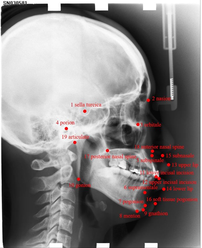
Appl. Sci. 2020, 10, 2547 6 of 16
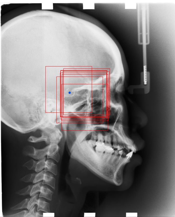
Figure 5. In the image, we take the reference image’s landmarks(Training images) as center of the patch
image, then we draw a bounding box (ROI) in the test image, as the input to our corresponding trained
models. Red dots are the reference images’ landmarks, green dots are test image’s landmarks, which
are the landmarks we aim to detect.
Figure 6. The architecture of Automatic registration.
3.3. Landmark Detection
3.3.1. Network Architecture
We use the ResNet50 architecture [24] as our backbone to extract features in ROI patches. CNN
can extract useful features automatically for different computer vision tasks. We use regression method
to estimate the landmark location after feature extraction. In our experiment, we choose to use fully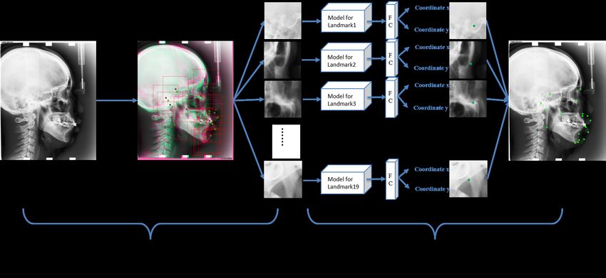
Appl. Sci. 2020, 10, 2547                                                                                       7 of 16

connected layer for the estimation of landmark location as a regression problem. We first flatten all
the features. Then, we add one fully connected layer, which directly outputs the coordinate of the
landmark in the patch.
     The state-of-the-art architecture ResNet is widely used for its unique architecture. It has
convolutional blocks and identity blocks. By adding former information to the later layers, ResNet
solves the gradient vanishing problems effectively. The overall architecture of ResNet50 is presented
in Figure 7.

      Figure 7. The architecture of ResNet50, the identity block and convolutional block add the former
      input to the later output. For identity block, it directly adds the former input to the later output. While
      for convolutional block, before adding, the former input first goes through a convolutional layer to
      make it the same size with later output.

3.3.2. Cost function
     The cost function we used during training is mean squared error (MSE), since we want to make
the predicted landmark become as close as possible to the ground-truth landmark location during
training. In this case, MSE can be written as in Equation (1):
                                                    n
                                               1
                                     MSE =
                                               n   ∑ ((xi − x̂i )2 + (yi − ŷi )2 )                                 (1)
                                                   i =1

where xi and yi indicate the ground-truth coordinate, and x̂i and ŷi indicate the estimated coordinate.

4. Experiments and Discussion

4.1. Implementation
     For the implementation of our experiments, we use Titan X GPU (12 GB) to help accelerating
training. We use Python programming language along with deep learning tools Tensorflow and Keras
in our experiments. We use Adam optimizer and set learning rate to 0.001. Ten percent of our training
data (60,000 × 10% = 6000) are separated for validation during training procedure and early stopping
is applied to find the best weights.

4.2. Evaluation measures
     According to the 2015 ISBI challenges on cephalometry landmark detection [6], we use the mean
radial error (MRE) to make evaluation. The radial error is defined in Equation (2). ∆x and ∆y are the
absolute differences of the estimated coordinate and ground-truth coordinate of x-axis and y-axis.
                                               q
                                          R = ∆x2 + ∆y2                                            (2)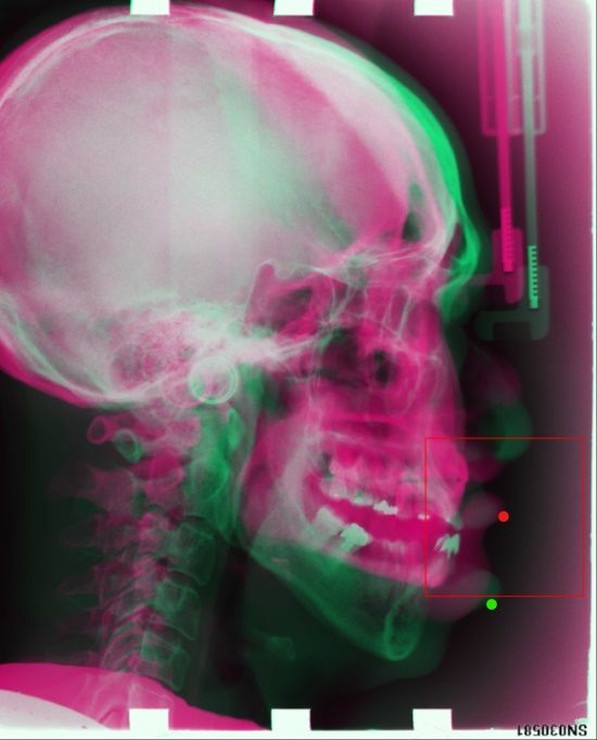
Appl. Sci. 2020, 10, 2547                                                                                      8 of 16

      The mean radial error (MRE) is defined in Equation (3):

                                                             ∑in=1 Ri
                                                   MRE =                                                          (3)
                                                                 n
     Because the predicted results have some difference with the ground-truth. If the difference is
within some range, we consider it correct in that range. In our experiment, we evaluate the range of z
mm (where z = 2, 2.5, 3, 4). For example, if the radial error is 1.5 mm, we consider it as a 2 mm success.
Equation (4) explains the meaning of successful detection rate (SDR), where Na indicates the number
of accurate detections, and N indicates total number of detections.

                                                            Na
                                                   SDR =       ∗ 100%                                             (4)
                                                            N

4.3. Landmark Detection Results

4.3.1. ISBI Test Dataset
     The results for ISBI public data are presented in Tables 1 and 2. Table 1 presents the SDR, and
Table 2 presents the MRE results.

      Table 1. Successful Detection Rate (SDR) Results on Testset1 and Testset2 of range 2 mm, 2.5 mm, 3 mm,
      4 mm.

                                          SDR (Successful Detection Rate)

  Anatomical Landmarks                2 mm (%)          2.5 mm (%)             3 mm (%)            4 mm (%)

                               Testset1 Testset2 Testset1 Testset2 Testset1 Testset2 Testset1 Testset2

  1. sella turcica             98.7        99.0      98.7       99.0    99.3        99.0    99.3        99.0
  2. nasion                    86.7        89.0      89.3       90.0    93.3        92.0    96.0        99.0
  3. orbitale                  84.7        36.0      92.0       61.0    96.0        80.0    99.3        96.0
  4. porion                    68.0        78.0      78.0       81.0    84.7        86.0    93.3        93.0
  5. subspinale                66.0        84.0      76.0       94.0    87.3        99.0    95.3        100.0
  6. supramentale              87.3        27.0      93.3       43.0    97.3        59.0    98.7        82.0
  7. pogonion                  93.3        98.0      97.3       100.0   98.7        100.0   99.3        100.0
  8. menton                    94.0        96.0      98.0       98.0    98.0        99.0    99.3        100.0
  9. gnathion                  94.0        100.0     98.0       100.0   98.0        100.0   99.3        100.0
  10. gonion                   62.7        75.0      75.3       87.0    84.7        94.0    92.0        98.0
  11. lower incisal incision   92.7        93.0      97.3       96.0    97.3        97.0    99.3        99.0
  12. upper incisal incision   97.3        95.0      98.0       98.0    98.7        98.0    99.3        98.0
  13. upper lip                89.3        13.0      98.0       35.0    99.3        69.0    99.3        93.0
  14. lower lip                99.3        63.0      99.3       80.0    100.0       93.0    100.0       98.0
  15. subnasale                92.7        92.0      95.3       94.0    96.7        95.0    99.3        99.0
  16. soft tissue pogonion     86.7        4.0       92.7       7.0     95.3        13.0    99.3        41.0
  17. posterior nasal spine    94.7        91.0      97.3       98.0    98.7        100.0   99.3        100.0
  18. anterior nasal spine     87.3        93.0      92.0       96.0    95.3        97.0    98.7        100.0
  19. articulate               66.0        80.0      76.0       87.0    83.0        93.0    91.3        97.0

  Average:                     86.4        74.0      91.7       81.3    94.8        87.5    97.8        94.3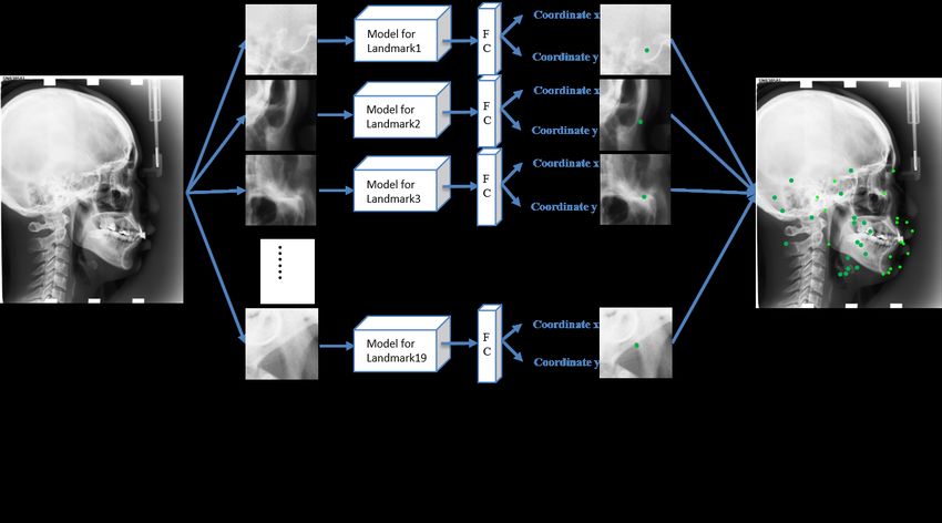
Appl. Sci. 2020, 10, 2547                                                                              9 of 16

                              Table 2. Results on Testset1 and Testset2 of mean radial error.

                                Anatomical Landmarks               Mean Radial Error (mm)

                                                                   Testset1   Testset2

                                1. sella turcica                   0.577      0.613
                                2. nasion                          1.133      0.981
                                3. orbitale                        1.243      2.356
                                4. porion                          1.828      1.702
                                5. subspinale                      1.752      1.253
                                6. supramentale                    1.136      2.738
                                7. pogonion                        0.836      0.594
                                8. menton                          0.952      0.705
                                9. gnathion                        0.952      0.594
                                10. gonion                         1.817      1.431
                                11. lower incisal incision         0.697      0.771
                                12. upper incisal incision         0.532      0.533
                                13. upper lip                      1.332      2.841
                                14. lower lip                      0.839      1.931
                                15. subnasale                      0.853      0.999
                                16. soft tissue pogonion           1.173      4.265
                                17. posterior nasal spine          0.819      1.028
                                18. anterior nasal spine           1.157      0.995
                                19. articulate                     1.780      1.310

                                Average:                           1.077      1.542

      We compare our detection results with other benchmarks’ results. Table 3 shows the comparison.

      Table 3. SDR of the proposed method compared with other benchmarks for ISBI 2015 challenges on
      cephalometry landmark detection Testset1 and Testset2.

                                                     Comparisons of SDR

                Method                             2 mm (%)      2.5 mm (%)     3 mm (%)    4 mm (%)

                                                            Testset1

                Ibrgimov(2015) [8]                 71.7          77.4           81.9        88.0
                Lindner [7]                        73.7          80.2           85.2        91.5
                Ibragimov [9]                      75.4          80.9           84.3        88.3
                Jiahong Qian [11]                  82.5          86.2           89.3        90.6
                Proposed:                          86.4          91.7           94.8        97.8

                                                            Testset2

                Ibrgimov [8]                       62.7          70.5           76.5        85.1
                Lindner [7]                        66.1          72.0           77.6        87.4
                Ibragimov [9]                      67.7          74.2           79.1        84.6
                Jiahong Qian [11]                  72.4          76.2           80.0        85.9
                Proposed:                          74.0          81.3           87.5        94.3

      Figure 8 shows one of the examples of our results.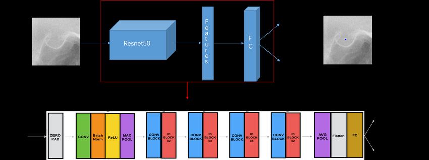
Appl. Sci. 2020, 10, 2547                                                                                    10 of 16

      Figure 8. Green points: predicted landmarks’ locations. Red points: ground-truth of landmarks’ locations.

4.3.2. Our Dataset
     We use our trained model(use ISBI training dataset) to test our own dataset directly. We also
register all images first. Since there are some different landmarks labeled in our own dataset, in the
experiment, we only test same parts’ landmarks with ISBI dataset. The results are presented in
Tables 4 and 5.

      Table 4. Results of 2 mm, 2.5 mm, 3 mm and 4 mm accuracy on our own dataset, since we do not have
      label for landmark 13, 14, 15, 16, 17, 19, we test other landmarks exclude these ones.

                                     Our own data from Shandong University

              Anatomical Landmarks            2 mm (%)       2.5 mm (%)     3 mm (%)       4 mm (%)

              1. sella turcica                68.0           71.0           76.0           82.0
              2. nasion                       83.0           90.0           95.0           99.0
              3. orbitale                     40.0           58.0           74.0           88.0
              4. porion                       48.0           56.0           66.0           72.0
              5. subspinale                   32.0           39.0           50.0           67.0
              6. supramentale                 33.0           43.0           55.0           71.0
              7. pogonion                     68.0           77.0           81.0           90.0
              8. menton                       82.0           86.0           95.0           99.0
              9. gnathion                     91.0           97.0           99.0           100.0
              10.gonion                       51.0           63.0           75.0           86.0
              11.lower incisal incision       68.0           76.0           78.0           90.0
              12.upper incisal incision       75.0           86.0           90.0           97.0
              18.anterior nasal spine         67.0           74.0           81.0           85.0

              Average:                        62.0           70.5           78.1           86.6
Appl. Sci. 2020, 10, 2547 11 of 16
Table 5. Results of Mean Radial Error on our own dataset.
Our own data from Shandong University
Anatomical Landmarks Mean Radial Error (mm)
1. sella turcica 2.4
2. nasion 1.4
3. orbitale 2.5
4. porion 3.0
5. subspinale 3.6
6. supramentale 3.3
7. pogonion 1.7
8. menton 1.2
9. gnathion 1.2
10.gonion 2.4
11.lower incisal incision 1.8
12.upper incisal incision 1.3
18.anterior nasal spine 2.0
Average: 2.1
4.4. Skeletal Malformations Classification
For the ISBI Grand Challenge, the class labels of skeletal malformations based on ANB, SNB,
SNA, ODI, APDI, FHI, FMA, and MW were also annotated for each subject. The skeletal malformation
classifications for ANB, SNB, SNA, ODI, APDI, FHI, FMA, and MW are defined in Table 6 and the
definitions (calculations) of ANB, SNB, SNA, ODI, APDI, FHI, FMA, and MW are summarized as
follows:
1. ANB: The angle between Landmark 5, Landmark 2 and Landmark 6
2. SNB: The angle between Landmark 1, Landmark 2 and Landmark 6
3. SNA: The angle between Landmark 1, Landmark 2 and Landmark 5
4. ODI (Overbite Depth Indicator): Sum of the angle between the lines from Landmark 5 to
Landmark 6 and from Landmark 8 to Landmark 10 and the angle between the lines from
Landmark 3 to Landmark 4 and from Landmark 17 to Landmark 18
5. APDI (AnteroPosterior Dysplasia Indicator): Sum of the angle between the lines from Landmark 3
to Landmark 4 and from Landmark 2 to Landmark 7, the angle between the lines from Landmark
2 to Landmark 7 and from Landmark 5 to Landmark 6 and the angle between the lines from
Landmark 3 to Landmark 4 and from Landmark 17 to Landmark 18
6. FHI: Obtained by the ratio of the Posterior Face Height (PFH = the distance from Landmark 1 to
Landmark 10) to the Anterior Face Height (AFH = the distance from Landmark 2 to Landmark 8).
FHI = PFH/AFH.
7. FMA: The angle between the line from Landmark 1 to Landmark 2 and the line from Landmark
10 to Landmark 9.
8. Modify-Wits (MW): The distance between Landmark 12 and Landmark 11.
q
MW = ( x L12 − x L11 )2 + (y L12 − y L11 )2 .Appl. Sci. 2020, 10, 2547 12 of 16
Table 6. Classifications for 8 methods, ANB, SNB, SNA, ODI, APDI, FHI, FMA and MW.
ANB SNB SNA ODI APDI FHI FMA MW
Class1 (C1) 3.2◦ –5.7◦ 74.6◦ –78.7◦ 79.4◦ –83.2◦ 68.4◦ –80.5◦ 77.6◦ –85.2◦ 0.65–0.75 26.8◦ –31.4◦ 2–4.5 mm
Class2 (C2) >5.7◦ 83.2◦ >80.5◦ 0.75 >31.4◦ =0 mm
Class3 (C3) 78.7◦Appl. Sci. 2020, 10, 2547 13 of 16
junior doctor. If we used the annotation data of the senior doctor as the ground truth when performing
classification, the SCR would be lower. It proves that annotation data have great influence on the
results. During training, we use the average of the annotated landmark locations of the two doctors as
the ground truth. When we use only the senior doctor’s annotated landmark locations as the ground
truth during the training, the SDR would also drop, which also proves that the annotation data greatly
affects the final results.
Table 8. The proportion that two doctors made the same classification label over 400 images (training
and test images).
Proportion (%)
ANB SNB SNA ODI APDI FHI FMA MW
78.0 82.0 67.75 77.0 82.25 84.25 82.0 87.5
Figure 9. Green point: test image’s landmark location. Red point: reference image’s landmark location.
We can see that the green dot is not included in the bounding box we cropped.
Figure 10. Successful detection example from Testset1 and failed detection example from Testset2 on
Landmark 3. Green points: predicted result. Blue points: ground-truth location.Appl. Sci. 2020, 10, 2547 14 of 16
Figure 11. Green points: predicted landmarks’ locations. Red points: ground-truth locations of
landmarks. We can see the result is not satisfying at all.
5. Conclusions
We proposed an approach to automatically predict landmark location and used a deep learning
method with very small training data, with only 150 X-ray training images. The results outperformed
other benchmarks’ results in all SDR and nearly all SCR, which proves that the proposed method are
effective for cephalometric landmark detection. The proposed method could be used for landmark
detection in clinical practice under the supervision of doctors.
For future work, we are developing a GUI for doctors to use. The system offers either automatic
or semi-automatic landmark detection. In the automatic mode, the system will automatically extract an
ROI (based on registration) and select a proper model for each landmark. In the semi-automatic mode,
the doctor needs to give a bounding box extract ROI manually and select a corresponding model for
each landmark detection, which can reduce computational time. Since we used simple registration
in this study and it took a long time to register one test image with all the training images, around
twenty minutes as we mentioned before. Under such case, we aim to design a better method that
reduces the registration time in testing phase, to make the automatic detection more efficient. For
example, maybe we will also utilize deep learning method, either to do registration or just simply to
regress a coarse landmark region, to replace the rigid registration we used in this paper. Moreover,
because we detected all the landmarks in patch images, we did not take global-context information
(i.e., the relationship among all the landmarks) into consideration. In future work, we want to utilize
this global-context information to check whether we can achieve better performance. For example,
maybe we will try to change the network architecture to allow the network to utilize whole image’s
features to better and faster locate the coarse locations of landmarks.
Author Contributions: Conceptualization, Y.S.; Data curation, Y.S. and X.Q.; Formal analysis, Y.S.; Funding
acquisition, X.Q. and Y.-w.C.; Investigation, Y.S.; Methodology, Y.S., X.Q., Y.I. and Y.-w.C.; Project administration,
X.Q.; Supervision, Y.I. and Y.-w.C.; Validation, Y.S.; Writing—original draft, Y.S.; Writing—review and editing, Y.S.,
X.Q., Y.I. and Y.-w.C. All authors have read and agreed to the published version of the manuscript.
Funding: This work was supported in part by the National Natural Science Foundation of China under the Grant
No. 61603218, and in part by the Grant-in Aid for Scientific Research from the Japanese Ministry for Education,
Science, Culture and Sports (MEXT) under the Grant No. 18H03267 and No. 17K00420.
Conflicts of Interest: The authors declare no conflict of interest.Appl. Sci. 2020, 10, 2547 15 of 16
Abbreviations
The following abbreviations are used in this manuscript:
GUI The graphical user interface
SCR Successful Classification Rate
SDR Successful Detection Rate
MRE Mean squared error
ROI Region of interest
References
1. Kaur, A.; Chandan Singh, T. Automatic cephalometric landmark detection using Zernike moments and
template matching. Signal Image Video Process. 2015, 29, 117–132. [CrossRef]
2. Grau, V.; Alcaniz, M.; Juan, M.C.; Monserrat, C.; Knol, T. Automatic localization of cephalometric landmarks.
J. Biomed. Inform. 2001, 34, 146–156. [CrossRef]
3. Ferreira, J.T.L.; Carlos de Souza Telles, T. Evaluation of the reliability of computerized profile cephalometric
analysis. Braz. Dent. J. 2002, 13, 201–204. [CrossRef] [PubMed]
4. Weining, Y.; Yin, D.; Li, C.; Wang, G.; Tianmin, X.T. Automated 2-D cephalometric analysis on X-ray images
by a model-based approach. IEEE Trans. Biomed. Eng. 2006, 13, 1615–1623. [CrossRef] [PubMed]
5. Ching-Wei, W.; Huang, C.; Hsieh, M.; Li, C.; Chang, S.; Li, W.; Vandaele, R. Evaluation and comparison of
anatomical landmark detection methods for cephalometric X-ray images: A grand challenge. IEEE Trans.
Biomed. Eng. 2015, 53, 1890–1900.
6. Wang, C.W.; Huang, C.T.; Lee, J.H.; Li, C.H.; Chang, S.W.; Siao, M.J.; Lai, T.M.; Ibragimov, B.; Vrtovec, T.;
Ronneberger, O.; et al. A benchmark for comparison of dental radiography analysis algorithms. IEEE Trans.
Biomed. Eng. 2016, 31, 63–76. [CrossRef] [PubMed]
7. Lindner, C.; Tim, F.; Cootes, T. Fully automatic cephalometric evaluation using Random Forest
regression-voting. In Proceedings of the IEEE International Symposium on Biomedical Imaging (ISBI),
Brooklyn Bridge, NY, USA, 16–19 April 2015.
8. Ibragimov, B.; Boštjan, L.; Pernus, F.; Tomaž Vrtovec, T. Computerized cephalometry by game theory with
shape-and appearance-based landmark refinement. In Proceedings of the IEEE International Symposium
on Biomedical Imaging (ISBI), Brooklyn Bridge, NY, USA, 16–19 April 2015.
9. Arik, S.Ö.; Bulat, I.; Lei, X.T. Fully automated quantitative cephalometry using convolutional neural networks.
J. Med. Imaging 2017, 4, 014501
10. Lee, H.; Park, M.; Kim, J. Cephalometric landmark detection in dental x-ray images using convolutional
neural networks. In Proceedings of the Medical Imaging 2017: Computer-Aided Diagnosis, Orlando, FL,
USA, 3 March 2017.
11. Qian, J.; Cheng, M.; Tao, Y.; Lin, J.; Lin, H. CephaNet: An Improved Faster R-CNN for Cephalometric
Landmark Detection. In Proceedings of the 2019 IEEE 16th International Symposium on Biomedical Imaging
(ISBI 2019), Venice, Italy, 8–11 April 2019; pp. 868–871.
12. Ren, S.; He, K.; Girshick, R; Sun, J., Faster r-cnn: Towards real-time object detection with region proposal
networks. In Proceedings of the Advances in neural information processing systems(NIPS), Montreal, QC,
Canada, 7–12 December 2015; pp. 91–99.
13. Ramanan, D.; Zhu, T. Face detection, pose estimation, and landmark localization in the wild. In Proceedings
of the 2012 IEEE Conference on Computer Vision and Pattern Recognition (CVPR), Providence, RI, USA,
16–21 June 2012; pp. 2879–2886.
14. Belhumeur, P.N.; David, W.; David, J.; Kriegman, J.; Neeraj Kumar, T. Localizing parts of faces using a
consensus of exemplars. IEEE Trans. Pattern Anal. Mach. Intell. 2013, 35, 2930–2940. [CrossRef] [PubMed]
15. Simonyan, K.; Andrew, Z.T. Very deep convolutional networks for large-scale image recognition. arXiv 2014,
arXiv:1409.1556.
16. Krizhevsky, A.; Ilya, S.; Geoffrey, E.; Hinton, T. Imagenet classification with deep convolutional neural
networks. Adv. Neural Inf. Process. Syst. 2012, 1097–1105. [CrossRef]Appl. Sci. 2020, 10, 2547 16 of 16
17. Claudiu, C.D.; Meier, U.; Masci, J.; Gambardella, L.M.; Schmidhuber, J. Flexible, High Performance
Convolutional Neural Networks for Image Classification. In Proceedings of the Twenty-Second International
Joint Conference on Artificial Intelligence, Barcelona, Spain, 16–22 July 2011.
18. Long, J.; Shelhamer, E.; Darrell, T. Fully Convolutional Networks for Semantic Segmentation. In Proceedings
of the IEEE Conference on Computer Vision and Pattern Recognition (CVPR), Boston, MA, USA,
7–12 June 2015; pp. 3431–3440.
19. Olaf, R.; Fischer, P.; Brox, T. U-net: Convolutional networks for biomedical image segmentation.
In Proceedings of the International Conference on Medical image computing and computer-assisted
intervention, Munich, Germany, 5–9 October 2015; pp. 234–241.
20. Pfister, T.; Charles, J.; Zisserman, A. Flowing convnets for human pose estimation in videos. In Proceedings
of the IEEE International Conference on Computer Vision (ICCV), Santiago, Chile, 13–16 December 2015.
21. Payer, C.; Štern, D.; Bischof, H.; Urschler, M. Regressing heatmaps for multiple landmark localization using
CNNs. In Proceedings of the International Conference on Medical Image Computing and Computer-Assisted
Intervention (MICCAI). Athens, Greece, 17–21 October 2016.
22. Davison, A. K.; Lindner, C.; Perry, D. C.; Luo, W.; Cootes, T. F. Landmark localisation in radiographs using
weighted heatmap displacement voting. In Proceedings of the International Workshop on Computational
Methods and Clinical Applications in Musculoskeletal Imaging (MSKI), Granada, Spain, 16 September 2018;
pp. 73–85.
23. Tompson, J. J.; Jain, A.; LeCun, Y.; Bregler, C. Joint training of a convolutional network and a graphical model
for human pose estimation. In Proceedings of the Advances in neural information processing systems
(NIPS), Montreal, QC, Canada, 8–13 December 2014; pp. 1799–1807.
24. Kaiming, H.; Zhang, X.; Ren, S.; Sun, J. Deep residual learning for image recognition. In Proceedings of the
IEEE Conference on Computer Vision and Pattern Recognition (CVPR), Las Vegas, NV, USA, 27–30 June 2016;
pp. 770–778.
c 2020 by the authors. Licensee MDPI, Basel, Switzerland. This article is an open access
article distributed under the terms and conditions of the Creative Commons Attribution
(CC BY) license (http://creativecommons.org/licenses/by/4.0/).You can also read