Projective dictionary pair learning for pattern classification
←
→
Page content transcription
If your browser does not render page correctly, please read the page content below
Projective dictionary pair learning for pattern
                         classification

                  Shuhang Gu1 , Lei Zhang1 , Wangmeng Zuo2 , Xiangchu Feng3
         1
           Dept. of Computing, The Hong Kong Polytechnic University, Hong Kong, China
    2
      School of Computer Science and Technology, Harbin Institute of Technology, Harbin, China
                  3
                    Dept. of Applied Mathematics, Xidian University, Xi0 an, China
                         {cssgu, cslzhang}@comp.polyu.edu.hk
                  cswmzuo@gmail.com, xcfeng@mail.xidian.edu.cn

                                             Abstract

         Discriminative dictionary learning (DL) has been widely studied in various pattern
         classification problems. Most of the existing DL methods aim to learn a synthesis
         dictionary to represent the input signal while enforcing the representation coef-
         ficients and/or representation residual to be discriminative. However, the `0 or
         `1 -norm sparsity constraint on the representation coefficients adopted in most DL
         methods makes the training and testing phases time consuming. We propose a new
         discriminative DL framework, namely projective dictionary pair learning (DPL),
         which learns a synthesis dictionary and an analysis dictionary jointly to achieve
         the goal of signal representation and discrimination. Compared with convention-
         al DL methods, the proposed DPL method can not only greatly reduce the time
         complexity in the training and testing phases, but also lead to very competitive
         accuracies in a variety of visual classification tasks.

1    Introduction

Sparse representation represents a signal as the linear combination of a small number of atoms cho-
sen out of a dictionary, and it has achieved a big success in various image processing and computer
vision applications [1, 2]. The dictionary plays an important role in the signal representation process
[3]. By using a predefined analytical dictionary (e.g., wavelet dictionary, Gabor dictionary) to rep-
resent a signal, the representation coefficients can be produced by simple inner product operations.
Such a fast and explicit coding makes analytical dictionary very attractive in image representation;
however, it is less effective to model the complex local structures of natural images.
Sparse representation with a synthesis dictionary has been widely studied in recent years [2, 4, 5].
With synthesis dictionary, the representation coefficients of a signal are usually obtained via an
`p -norm (p ≤1) sparse coding process, which is computationally more expensive than analytical
dictionary based representation. However, synthesis based sparse representation can better model
the complex image local structures and it has led to many state-of-the-art results in image restoration
[6]. Another important advantage lies in that the synthesis based sparse representation model allows
us to easily learn a desired dictionary from the training data. The seminal work of KSVD [1] tells
us that an over-complete dictionary can be learned from example natural images, and it can lead
to much better image reconstruction results than the analytically designed off-the-shelf dictionaries.
Inspired by KSVD, many dictionary learning (DL) methods have been proposed and achieved state-
of-the-art performance in image restoration tasks.
The success of DL in image restoration problems triggers its applications in image classification
tasks. Different from image restoration, assigning the correct class label to the test sample is the
goal of classification problems; therefore, the discrimination capability of the learned dictionary is

                                                  1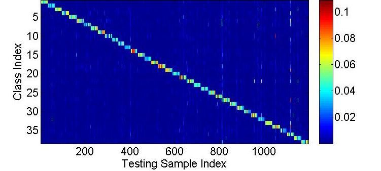
of the major concern. To this end, supervised dictionary learning methods have been proposed to
promote the discriminative power of the learned dictionary [4, 5, 7, 8, 9]. By encoding the query
sample over the learned dictionary, both the coding coefficients and the coding residual can be used
for classification, depending on the employed DL model. Discriminative DL has led to many state-
of-the-art results in pattern recognition problems.
One popular strategy of discriminative DL is to learn a shared dictionary for all classes while en-
forcing the coding coefficients to be discriminative [4, 5, 7]. A classifier on the coding coefficients
can be trained simultaneously to perform classification. Mairal et al. [7] proposed to learn a dictio-
nary and a corresponding linear classifier in the coding vector space. In the label consistent KSVD
(LC-KSVD) method, Jiang et al. [5] introduced a binary class label sparse code matrix to encourage
samples from the same class to have similar sparse codes. In [4], Mairal et al. proposed a task driv-
en dictionary learning (TDDL) framework, which minimizes different risk functions of the coding
coefficients for different tasks.
Another popular line of research in DL attempts to learn a structured dictionary to promote dis-
crimination between classes [2, 8, 9, 10]. The atoms in the structured dictionary have class labels,
and the class-specific representation residual can be computed for classification. Ramirez et al. [8]
introduced an incoherence promotion term to encourage the sub-dictionaries of different classes
to be independent. Yang et al. [9] proposed a Fisher discrimination dictionary learning (FDDL)
method which applies the Fisher criterion to both representation residual and representation coef-
ficient. Wang et al. [10] proposed a max-margin dictionary learning (MMDL) algorithm from the
large margin perspective.
In most of the existing DL methods, `0 -norm or `1 -norm is used to regularize the representation
coefficients since sparser coefficients are more likely to produce better classification results. Hence
a sparse coding step is generally involved in the iterative DL process. Although numerous algorithms
have been proposed to improve the efficiency of sparse coding [11, 12], the use of `0 -norm or `1 -
norm sparsity regularization is still a big computation burden and makes the training and testing
inefficient.
It is interesting to investigate whether we can learn discriminative dictionaries but without the costly
`0 -norm or `1 -norm sparsity regularization. In particular, it would be very attractive if the represen-
tation coefficients can be obtained by linear projection instead of nonlinear sparse coding. To this
end, in this paper we propose a projective dictionary pair learning (DPL) framework to learn a syn-
thesis dictionary and an analysis dictionary jointly for pattern classification. The analysis dictionary
is trained to generate discriminative codes by efficient linear projection, while the synthesis dictio-
nary is trained to achieve class-specific discriminative reconstruction. The idea of using functions to
predict the representation coefficients is not new, and fast approximate sparse coding methods have
been proposed to train nonlinear functions to generate sparse codes [13, 14]. However, there are
clear difference between our DPL model and these methods. First, in DPL the synthesis dictionary
and analysis dictionary are trained jointly, which ensures that the representation coefficients can be
approximated by a simple linear projection function. Second, DPL utilizes class label information
and promotes discriminative power of the representation codes.
One related work to this paper is the analysis-based sparse representation prior learning [15, 16],
which represents a signal from a dual viewpoint of the commonly used synthesis model. Analy-
sis prior learning tries to learn a group of analysis operators which have sparse responses to the
latent clean signal. Sprechmann et al. [17] proposed to train a group of analysis operators for clas-
sification; however, in the testing phase a costly sparsity-constrained optimization problem is still
required. Feng et al. [18] jointly trained a dimensionality reduction transform and a dictionary
for face recognition. The discriminative dictionary is trained in the transformed space, and sparse
coding is needed in both the training and testing phases.
The contribution of our work is two-fold. First, we introduce a new DL framework, which extends
the conventional discriminative synthesis dictionary learning to discriminative synthesis and analysis
dictionary pair learning (DPL). Second, the DPL utilizes an analytical coding mechanism and it
largely improves the efficiency in both the training and testing phases. Our experiments in various
visual classification datasets show that DPL achieves very competitive accuracy with state-of-the-art
DL algorithms, while it is significantly faster in both training and testing.

                                                   2
2 Projective Dictionary Pair Learning
2.1 Discriminative dictionary learning
Denote by X = [X1 , . . . , Xk , . . . , XK ] a set of p-dimensional training samples from K classes, where
Xk ∈ Rp×n is the training sample set of class k, and n is the number of samples of each class. Dis-
criminative DL methods aim to learn an effective data representation model from X for classification
tasks by exploiting the class label information of training data. Most of the state-of-the-art discrim-
inative DL methods [5, 7, 9] can be formulated under the following framework:
minD,A k X − DA k2F +λ k A kp +Ψ(D, A, Y), (1)
where λ ≥ 0 is a scalar constant, Y represents the class label matrix of samples in X, D is the
synthesis dictionary to be learned, and A is the coding coefficient matrix of X over D. In the training
model (1), the data fidelity term k X − DA k2F ensures the representation ability of D; k A kp is
the `p -norm regularizer on A; and Ψ(D, A, Y) stands for some discrimination promotion function,
which ensures the discrimination power of D and A.
As we introduced in Section 1, some DL methods [4, 5, 7] learn a shared dictionary for all classes
and a classifier on the coding coefficients simultaneously, while some DL methods [8, 9, 10] learn
a structured dictionary to promote discrimination between classes. However, they all employ `0 or
`1 -norm sparsity regularizer on the coding coefficients, making the training stage and the consequent
testing stage inefficient.
In this work, we extend the conventional DL model in (1), which learns a discriminative synthesis
dictionary, to a novel DPL model, which learns a pair of synthesis and analysis dictionaries. No
costly `0 or `1 -norm sparsity regularizer is required in the proposed DPL model, and the coding
coefficients can be explicitly obtained by linear projection. Fortunately, DPL does not sacrifice the
classification accuracy while achieving significant improvement in the efficiency, as demonstrated
by our extensive experiments in Section 3.
2.2 The dictionary pair learning model
The conventional discriminative DL model in (1) aims to learn a synthesis dictionary D to sparsely
represent the signal X, and a costly `1 -norm sparse coding process is needed to resolve the code A.
Suppose that if we can find an analysis dictionary, denoted by P ∈ RmK×p , such that the code A
can be analytically obtained as A = PX, then the representation of X would become very efficient.
Based on this idea, we propose to learn such an analysis dictionary P together with the synthesis
dictionary D, leading to the following DPL model:
{P∗ ,D∗ } = arg min k X − DPX k2F +Ψ(D, P, X, Y), (2)
P,D
where Ψ(D, P, X, Y) is some discrimination function. D and P form a dictionary pair: the analysis
dictionary P is used to analytically code X, and the synthesis dictionary D is used to reconstruct X.
The discrimination power of the DPL model depends on the suitable design of Ψ(D, P, X, Y) .
We propose to learn a structured synthesis dictionary D = [D1 , . . . , Dk , . . . , DK ] and a structured
analysis dictionary P = [P1 ; . . . ; Pk ; . . . ; PK ], where {Dk ∈ Rp×m , Pk ∈ Rm×p } forms a sub-
dictionary pair corresponding to class k. Recent studies on sparse subspace clustering [19] have
proved that a sample can be represented by its corresponding dictionary if the signals satisfy certain
incoherence condition. With the structured analysis dictionary P, we want that the sub-dictionary
Pk can project the samples from class i, i 6= k, to a nearly null space, i.e.,
Pk Xi ≈ 0, ∀k 6= i. (3)
Clearly, with (3) the coefficient matrix PX will be nearly block diagonal. On the other hand, with
the structured synthesis dictionary D, we want that the sub-dictionary Dk can well reconstruct the
data matrix Xk from its projective code matrix Pk Xk ; that is, the dictionary pair should minimize
the reconstruction error: XK
min k Xk − Dk Pk Xk k2F . (4)
P,D k=1
Based on the above analysis, we can readily have the following DPL model:
XK
{P∗ , D∗ } = arg min k Xk − Dk Pk Xk k2F +λ k Pk X̄k k2F , s.t. k di k22 ≤ 1. (5)
P,D k=1
3Algorithm 1 Discriminative synthesis&analysis dictionary pair learning (DPL)
Input: Training samples for K classes X = [X1 , X2 , . . . , XK ], parameter λ, τ , m;
1: Initialize D(0) and P(0) as random matrixes with unit Frobenious norm, t = 0;
2: while not converge do
3: t ← t + 1;
4: for i=1:K do
(t)
5: Update Ak by (8);
(t)
6: Update Pk by (10);
(t)
7: Update Dk by (12);
8: end for
9: end while
Output: Analysis dictionary P, synthesis dictionary D.
where X̄k denotes the complementary data matrix of Xk in the whole training set X, λ > 0 is a scalar
constant, and di denotes the ith atom of synthesis dictionary D. We constrain the energy of each
atom di in order to avoid the trivial solution of Pk = 0 and make the DPL more stable.
The DPL model in (5) is not a sparse representation model, while it enforces group sparsity on the
code matrix PX (i.e., PX is nearly block diagonal). Actually, the role of sparse coding in classifi-
cation is still an open problem, and some researchers argued that sparse coding may not be crucial
to classification tasks [20, 21]. Our findings in this work are supportive to this argument. The D-
PL model leads to very competitive classification performance with those sparse coding based DL
models, but it is much faster.
2.3 Optimization
The objective function in (5) is generally non-convex. We introduce a variable matrix A and relax
(5) to the following problem:
K
X
{P∗ , A∗ , D∗ } = arg min k Xi −Dk Ak k2F +τ k Pk Xk −Ak k2F +λ k Pk X̄k k2F , s.t. k di k22 ≤ 1. (6)
P,A,D
k=1
where τ is a scalar constant. All terms in the above objective function are characterized by Frobenius
norm, and (6) can be easily solved. We initialize the analysis dictionary P and synthesis dictionary
D as random matrices with unit Frobenius norm, and then alternatively update A and {D, P}. The
minimization can be alternated between the following two steps.
(1) Fix D and P, update A
XK
A∗ = arg min k Xk − Dk Ak k2F +τ k Pk Xk − Ak k2F . (7)
A k=1
This is a standard least squares problem and we have the closed-form solution:
A∗k = (DTk Dk + τ I)−1 (τ Pk Xk + DTk Xk ). (8)
(2) Fix A, update D and P:
( PK
P∗ = arg minP k=1 τ k Pk Xk − Ak k2F +λ k Pk X̄k k2F ;
PK (9)
D∗ = arg minD k=1 k Xk − Dk Ak k2F , s.t. k di k22 ≤ 1.
The closed-form solutions of P can be obtained as:
P∗k = τ Ak XTk (τ Xk XTk + λX̄k X¯Tk + γI)−1 , (10)
−4
where γ = 10e is a small number. The D problem can be optimized by introducing a variable S:
XK
min k Xk − Dk Ak k2F , s.t. D = S, k si k22 ≤ 1. (11)
D,S k=1
The optimal solution of (11) can be obtained by the ADMM algorithm:
PK (r) (r)
(r+1)
D
= arg minD k=1 k Xk − Dk Ak k2F +ρ k Dk − Sk + T k k2F ,
(r+1) PK (r+1) (r) 2
S = arg minS k=1 ρ k Dk − Sk + T k kF , s.t. k si k22 ≤ 1, (12)
(r+1) (r+1) (r+1)
T = T (r) + Dk − Sk , update ρ if appropriate.
42 2 ∗2 ∗2
(a)k P∗k P
(a)(a) y kPy22 y
* *
y yDyk −
(b)(b)(b)k PD
k k k2
2
yPk Pyk y k2
* ** *
D
k k 2 2 2
Figure 1: (a) The representation codes and (b) reconstruction error on the Extended YaleB dataset.
In each step of optimization, we have closed form solutions for variables A and P, and the ADMM
based optimization of D converges rapidly. The training of the proposed DPL model is much faster
than most of previous discriminative DL methods. The proposed DPL algorithm is summarized in
Algorithm 1. When the difference between the energy in two adjacent iterations is less than 0.01,
the iteration stops. The analysis dictionary P and the synthesis dictionary D are then output for
classification.
One can see that the first sub-objective function in (9) is a discriminative analysis dictionary learner,
focusing on promoting the discriminative power of P; the second sub-objective function in (9) is a
representative synthesis dictionary learner, aiming to minimize the reconstruction error of the input
signal with the coding coefficients generated by the analysis dictionary P. When the minimization
process converges, a balance between the discrimination and representation power of the model can
be achieved.
2.4 Classification scheme
In the DPL model, the analysis sub-dictionary P∗k is trained to produce small coefficients for samples
from classes other than k, and it can only generate significant coding coefficients for samples from
class k. Meanwhile, the synthesis sub-dictionary D∗k is trained to reconstruct the samples of class k
from their projective coefficients P∗k Xk ; that is, the residual k Xk − D∗k P∗k Xk k2F will be small. On
the other hand, since P∗k Xi , i 6= k, will be small and D∗k is not trained to reconstruct Xi , the residual
k Xi − D∗k P∗k Xi k2F will be much larger than k Xk − D∗k P∗k Xk k2F .
In the testing phase, if the query sample y is from class k, its projective coding vector by P∗k (i.e.,
P∗k y ) will be more likely to be significant, while its projective coding vectors by P∗i , i 6= k, tend to
be small. Consequently, the reconstruction residual k y − D∗k P∗k y k22 tends to be much smaller than
the residuals k y − D∗i P∗i y k22 , i 6= k. Let us use the Extended YaleB face dataset [22] to illustrate
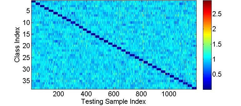
this. (The detailed experimental setting can be found in Section 3.) Fig. 1(a) shows the `2 -norm
of the coefficients P∗k y, where the horizontal axis refers to the index of y and the vertical axis refers
to the index of P∗k . One can clearly see that k P∗k y k22 has a nearly block diagonal structure, and
the diagonal blocks are produced by the query samples which have the same class labels as P∗k .
Fig. 1(b) shows the reconstruction residual k y − D∗k P∗k y k22 . One can see that k y − D∗k P∗k y k22 also
has a block diagonal structure, and only the diagonal blocks have small residuals. Clearly, the class-
specific reconstruction residual can be used to identify the class label of y, and we can naturally have
the following classifier associated with the DPL model:
identity(y) = arg mini k y − Di Pi y k2 . (13)
2.5 Complexity and Convergence
Complexity In the training phase of DPL, Ak , Pk and Dk are updated alternatively. In each iteration,
the time complexities of updating Ak , Pk and Dk are O(mpn + m3 + m2 n), O(mnp + p3 + mp2 ) and
O(W(pmn + m3 + m2 p + p2 m)), respectively, where W is the iteration number in ADMM algorithm
for updating D. We experimentally found that in most cases W is less than 20. In many applications,
the number of training samples and the number of dictionary atoms for each class are much smaller
than the dimension p. Thus the major computational burden in the training phase of DPL is on
T
updating Pk , which involves an inverse of a p × p matrix {τ Xk XTk + λX̄k X̄k + γI}. Fortunately, this
56
Energy
5
4
0 10 20 30 40 50
Iteration Number
Figure 2: The convergence curve of DPL on the AR database.
matrix will not change in the iteration, and thus the inverse of it can be pre-computed. This greatly
accelerates the training process.
In the testing phase, our classification scheme is very efficient. The computation of class-specific
reconstruction error k y − D∗k P∗k y k2 only has a complexity of O(mp). Thus, the total complexity of
our model to classify a query sample is O(Kmp).
Convergence The objective function in (6) is a bi-convex problem for {(D, P), (A)}, e.g., by fixing
A the function is convex for D and P, and by fixing D and P the function is convex for A. The con-
vergence of such a problem has already been intensively studied [23], and the proposed optimization
algorithm is actually an alternate convex search (ACS) algorithm. Since we have the optimal solu-
tions of updating A, P and D, and our objective function has a general lower bound 0, our algorithm
is guaranteed to converge to a stationary point. A detailed convergence analysis can be found in our
supplementary file.
It is empirically found that the proposed DPL algorithm converges rapidly. Fig. 2 shows the conver-
gence curve of our algorithm on the AR face dataset [24]. One can see that the energy drops quickly
and becomes very small after 10 iterations. In most of our experiments, our algorithm will converge
in less than 20 iterations.
3 Experimental Results
We evaluate the proposed DPL method on various visual classification datasets, including two face
databases (Extended YaleB [22] and AR [24]), one object categorization database (Caltech101)
[25], and one action recognition database (UCF 50 action [26]). These datasets are widely used in
previous works [5, 9] to evaluate the DL algorithms.
Besides the classification accuracy, we also report the training and testing time of competing algo-
rithms in the experiments. All the competing algorithms are implemented in Matlab except for SVM
which is implemented in C. All experiments are run on a desktop PC with 3.5GHz Intel CPU and
8 GB memory. The testing time is calculated in terms of the average processing time to classify a
single query sample.
3.1 Parameter setting
There are three parameters, m, λ and τ in the proposed DPL model. To achieve the best performance,
in face recognition and object recognition experiments, we set the number of dictionary atoms as
its maximum (i.e., the number of training samples) for all competing DL algorithms, including the
proposed DPL. In the action recognition experiment, since the samples per class is relatively big, we
set the number of dictionary atoms of each class as 50 for all the DL algorithms. Parameter τ is an
algorithm parameter, and the regularization parameter λ is to control the discriminative property of
P. In all the experiments, we choose λ and τ by 10-fold cross validation on each dataset. For all the
competing methods, we tune their parameters for the best performance.
3.2 Competing methods
We compare the proposed DPL method with the following methods: the base-line nearest subspace
classifier (NSC) and linear support vector machine (SVM), sparse representation based classification
(SRC) [2] and collaborative representation based classification (CRC) [21], and the state-of-the-art
DL algorithms DLSI [8], FDDL [9] and LC-KSVD [5]. The original DLSI represents the test sample
by each class-specific sub-dictionary. The results in [9] have shown that by coding the test sample
collaboratively over the whole dictionary, the classification performance can be greatly improved.
6(a) (b)
Figure 3: Sample images in the (a) Extended YaleB and (b) AR databases.
Therefore, we follow the use of DLDI in [9] and denote this method as DLSI(C). For the two
variants of LC-KSVD proposed in [5], we adopt the LC-KSVD2 since it can always produce better
classification accuracy.
3.3 Face recognition
We first evaluate our algorithm on two widely used face datasets: Extended YaleB [22] and AR [24].
The Extended YaleB database has large variations in illumination and expressions, as illustrated in
Fig. 3(a). The AR database (a)
involves many variations such as illumination, expressions and sunglass
and scarf occlusion, as illustrated in Fig. 3(b).
We follow the experimental settings in [5] for fair comparison with state-of-the-arts. A set of 2,414
face images of 38 persons are extracted from the Extended YaleB database. We randomly select half
of the images per subject for training and the other half for testing. For the AR database, a set of
2,600 images of 50 female and 50 male subjects are extracted. 20 images of each subject are used
for training and the remain 6 images are used for testing. We use the features provided by Jiang
et al. [5] to represent the face image. The feature dimension is 504 for Extended YaleB and 540
for AR. The parameter τ is set to 0.05 on both the datasets and λ is set to 3e-3 and 5e-3 on the
Extended YaleB and AR datasets, respectively. In these two experiments, we also compare with the
max-margin dictionary learning (MMDL) [10] algorithm, whose recognition accuracy is cropped
from the original paper but the training/testing time is not available.
Table 1: Results on the Extended YaleB database. Table 2: Results on the AR database.
Accuracy Training Testing Accuracy Training Testing
(%) time (s) time (s) (%) time (s) time (s)
NSC 94.7 no need 1.41e-3 NSC 92.0 no need 3.29e-3
SVM 95.6 0.70 3.49e-5 SVM 96.5 3.42 6.16e-5
CRC 97.0 no need 1.92e-3 CRC 98.0 no need 5.08e-3
SRC 96.5 no need 2.16e-2 SRC 97.5 no need 3.42e-2
DLSI(C) 97.0 567.47 4.30e-2 DLSI(C) 97.5 2,470.5 0.16
FDDL 96.7 6,574.6 1.43 FDDL 97.5 61,709 2.50
LC-KSVD 96.7 412.58 4.22e-4 LC-KSVD 97.8 1,806.3 7.72e-4
MMDL 97.3 - - MMDL 97.3 - -
DPL 97.5 4.38 1.71e-4 DPL 98.3 11.30 3.93e-4
Extended YaleB database The recognition accuracies and training/testing time by different algo-
rithms on the Extended YaleB database are summarized in Table 1. The proposed DPL algorithm
achieves the best accuracy, which is slightly higher than MMDL, DLSI(C), LC-KSVD and FDDL.
However, DPL has obvious advantage in efficiency over the other DL algorithms.
AR database The recognition accuracies and running time on the AR database are shown in Table 2.
DPL achieves the best results among all the competing algorithms. Compared with the experiment
on Extended YaleB, in this experiment there are more training samples and the feature dimension is
higher, and DPL0 s advantage of efficiency is much more obvious. In training, it is more than 159
times faster than DLSI and LC-KSVD, and 5,460 times faster than FDDL.
3.4 Object recognition
In this section we test DPL on object categorization by using the Caltech101 database [25]. The
Caltech101 database [25] includes 9,144 images from 102 classes (101 common object classes and
a background class). The number of samples in each category varies from 31 to 800. Following
the experimental settings in [5, 27], 30 samples per category are used for training and the rest are
7Table 3: Recognition accuracy(%) & running time(s) on the Caltech101 database.
Accuracy Training time Testing time
NSC 70.1 no need 1.79e-2
SVM 64.6 14.6 1.81e-4
CRC 68.2 no need 1.38e-2
SRC 70.7 no need 1.09
DLSI(C) 73.1 97,200 1.46
FDDL 73.2 104,000 12.86
LC-KSVD 73.6 12,700 4.17e-3
DPL 73.9 134.6 1.29e-3
used for testing. We use the standard bag-of-words (BOW) + spatial pyramid matching (SPM)
framework [27] for feature extraction. Dense SIFT descriptors are extracted on three grids of sizes
1×1, 2×2, and 4×4 to calculate the SPM features. For a fair comparison with [5], we use the vector
quantization based coding method to extract the mid-level features and use the standard max pooling
approach to build up the high dimension pooled features. Finally, the original 21,504 dimensional
data is reduced to 3,000 dimension by PCA. The parameters τ and λ used in our algorithm are 0.05
and 1e-4, respectively.
The experimental results are listed in Table 3. Again, DPL achieves the best performance. Though
its classification accuracy is only slightly better than the DL methods, its advantage in terms of
training/testing time is huge.
3.5 Action recognition
Action recognition is an important yet very challenging task and it has been attracting great research
interests in recent years. We test our algorithm on the UCF 50 action database [26], which includes
50 categories of 6,680 human action videos from YouTube. We use the action bank features [28]
and five-fold data splitting to evaluate our algorithm. For all the comparison methods, the feature
dimension is reduced to 5,000 by PCA. The parameters τ and λ used in our algorithm are both 0.01.
The results by different methods are reported in Table 4. Our DPL algorithm achieves much higher
accuracy than its competitors. FDDL has the second highest accuracy; however, it is 1,666 times
slower than DPL in training and 83,317 times slower than DPL in testing.
Table 4: Recognition accuracy(%) & running time(s) on the UCF50 action database
Methods Accuracy Training time Testing time
NSC 51.8 no need 6.11e-2
SVM 57.9 59.8 5.02e-4
CRC 60.3 no need 6.76e-2
SRC 59.6 no need 8.92
DLSI(C) 60.0 397,000 10.11
FDDL 61.1 415,000 89.15
LC-KSVD 53.6 9,272.4 0.12
DPL 62.9 249.0 1.07e-3
4 Conclusion
We proposed a novel projective dictionary pair learning (DPL) model for pattern classification tasks.
Different from conventional dictionary learning (DL) methods, which learn a single synthesis dictio-
nary, DPL learns jointly a synthesis dictionary and an analysis dictionary. Such a pair of dictionaries
work together to perform representation and discrimination simultaneously. Compared with previ-
ous DL methods, DPL employs projective coding, which largely reduces the computational burden
in learning and testing. Performance evaluation was conducted on publically accessible visual clas-
sification datasets. DPL exhibits highly competitive classification accuracy with state-of-the-art DL
methods, while it shows significantly higher efficiency, e.g., hundreds to thousands times faster than
LC-KSVD and FDDL in training and testing.
8References
[1] Aharon, M., Elad, M., Bruckstein, A.: K-svd: An algorithm for designing overcomplete dictionaries for
sparse representation. IEEE Trans. on Signal Processing, 54(11) (2006) 4311–4322
[2] Wright, J., Yang, A.Y., Ganesh, A., Sastry, S.S., Ma, Y.: Robust face recognition via sparse representation.
IEEE Transactions on Pattern Analysis and Machine Intelligence 31(2) (2009) 210–227
[3] Rubinstein, R., Bruckstein, A.M., Elad, M.: Dictionaries for sparse representation modeling. Proceedings
of the IEEE 98(6) (2010) 1045–1057
[4] Mairal, J., Bach, F., Ponce, J.: Task-driven dictionary learning. IEEE Trans. Pattern Anal. Mach. Intelli-
gence 34(4) (2012) 791–804
[5] Jiang, Z., Lin, Z., Davis, L.: Label consistent k-svd: learning a discriminative dictionary for recognition.
IEEE Trans. on Pattern Anal. Mach. Intelligence 35(11) (2013) 2651–2664
[6] Elad, M., Aharon, M.: Image denoising via sparse and redundant representations over learned dictionar-
ies. IEEE Transactions on Image Processing 15(12) (2006) 3736–3745
[7] Mairal, J., Bach, F., Ponce, J., Sapiro, G., Zisserman, A., et al.: Supervised dictionary learning. In: NIPS.
(2008)
[8] Ramirez, I., Sprechmann, P., Sapiro, G.: Classification and clustering via dictionary learning with struc-
tured incoherence and shared features. In: CVPR. (2010)
[9] Yang, M., Zhang, L., , Feng, X., Zhang, D.: Fisher discrimination dictionary learning for sparse repre-
sentation. In: ICCV. (2011)
[10] Wang, Z., Yang, J., Nasrabadi, N., Huang, T.: A max-margin perspective on sparse representation-based
classification. In: ICCV. (2013)
[11] Lee, H., Battle, A., Raina, R., Ng, A.Y.: Efficient sparse coding algorithms. In: NIPS. (2007)
[12] Hale, E.T., Yin, W., Zhang, Y.: Fixed-point continuation for `1 -minimization: Methodology and conver-
gence. SIAM Journal on Optimization 19(3) (2008) 1107–1130
[13] Gregor, K., LeCun, Y.: Learning fast approximations of sparse coding. In: ICML. (2010)
[14] Ranzato, M., Poultney, C., Chopra, S., Cun, Y.L.: Efficient learning of sparse representations with an
energy-based model. In: NIPS. (2006)
[15] Yunjin, C., Thomas, P., Bischof, H.: Learning l1-based analysis and synthesis sparsity priors using bi-
level optimization. NIPS workshop (2012)
[16] Elad, M., Milanfar, P., Rubinstein, R.: Analysis versus synthesis in signal priors. Inverse problems 23(3)
(2007) 947
[17] Sprechmann, P., Litman, R., Yakar, T.B., Bronstein, A., Sapiro, G.: Efficient supervised sparse analysis
and synthesis operators. In: NIPS. (2013)
[18] Feng, Z., Yang, M., Zhang, L., Liu, Y., Zhang, D.: Joint discriminative dimensionality reduction and
dictionary learning for face recognition. Pattern Recognition 46(8) (2013) 2134–2143
[19] Soltanolkotabi, M., Elhamifar, E., Candes, E.: Robust subspace clustering. arXiv preprint arX-
iv:1301.2603 (2013)
[20] Coates, A., Ng, A.Y.: The importance of encoding versus training with sparse coding and vector quanti-
zation. In: ICML. (2011)
[21] Zhang, L., Yang, M., Feng, X.: Sparse representation or collaborative representation: Which helps face
recognition? In: ICCV. (2011)
[22] Georghiades, A., Belhumeur, P., Kriegman, D.: From few to many: Illumination cone models for face
recognition under variable lighting and pose. IEEE Trans. Patt. Anal. Mach. Intel. 23(6) (2001) 643–660
[23] Gorski, J., Pfeuffer, F., Klamroth, K.: Biconvex sets and optimization with biconvex functions: a survey
and extensions. Mathematical Methods of Operations Research 66(3) (2007) 373–407
[24] Martinez, A., Benavente., R.: The ar face database. CVC Technical Report (1998)
[25] Fei-Fei, L., Fergus, R., Perona, P.: Learning generative visual models from few training examples: An in-
cremental bayesian approach tested on 101 object categories. Computer Vision and Image Understanding
106(1) (2007) 59–70
[26] Reddy, K.K., Shah, M.: Recognizing 50 human action categories of web videos. Machine Vision and
Applications 24(5) (2013) 971–981
[27] Lazebnik, S., Schmid, C., Ponce, J.: Beyond bags of features: Spatial pyramid matching for recognizing
natural scene categories. In: CVPR. (2006)
[28] Sadanand, S., Corso, J.J.: Action bank: A high-level representation of activity in video. In: CVPR.
(2012)
9You can also read