-SS3: a text classifier with dynamic n-grams for early risk detection over text
←
→
Page content transcription
If your browser does not render page correctly, please read the page content below
τ -SS3: a text classifier with dynamic n-grams for early risk detection over text
                                                                                 streams

                                                                     Sergio G. Burdissoa,b,∗, Marcelo Errecaldea , Manuel Montes-y-Gómezc
                                                    a Universidad Nacional de San Luis (UNSL), Ejército de Los Andes 950, San Luis, San Lius, C.P. 5700, Argentina
                                                                    b Consejo Nacional de Investigaciones Cientı́ficas y Técnicas (CONICET), Argentina
                                         c Instituto Nacional de Astrofı́sica, Óptica y Electrónica (INAOE), Luis Enrique Erro No. 1, Sta. Ma. Tonantzintla, Puebla, C.P. 72840,

                                                                                                             Mexico

                                         Abstract
arXiv:1911.06147v1 [cs.CL] 11 Nov 2019

                                         A recently introduced classifier, called SS3, has shown to be well suited to deal with early risk detection (ERD) problems
                                         on text streams. It obtained state-of-the-art performance on early depression and anorexia detection on Reddit in the
                                         CLEF’s eRisk open tasks. SS3 was created to naturally deal with ERD problems since: it supports incremental training
                                         and classification over text streams and it can visually explain its rationale. However, SS3 processes the input using a
                                         bag-of-word model lacking the ability to recognize important word sequences. This could negatively affect the classification
                                         performance and also reduces the descriptiveness of visual explanations. In the standard document classification field, it
                                         is very common to use word n-grams to try to overcome some of these limitations. Unfortunately, when working with
                                         text streams, using n-grams is not trivial since the system must learn and recognize which n-grams are important “on the
                                         fly”. This paper introduces τ -SS3, a variation of SS3 which expands the model to dynamically recognize useful patterns
                                         over text streams. We evaluated our model on the eRisk 2017 and 2018 tasks on early depression and anorexia detection.
                                         Experimental results show that τ -SS3 is able to improve both, existing results and the richness of visual explanations.
                                         Keywords: Early Text Classification. Dynamic Word N-Grams. Incremental Classification. SS3. Explainability. Trie.
                                         Digital Tree.

                                         1. Introduction                                                       aggressive text identification [4], depression detection [9, 8]
                                                                                                               or terrorism detection [6].
                                        The analysis of sequential data is a very active research                  ERD scenarios are difficult to deal with since models
                                    area that addresses problems where data is processed natu-                 need to support: classifications and/or learning over of
                                    rally as sequences or can be better modeled that way, such                 sequential data (streams); provide a clear method to decide
                                    as sentiment analysis, machine translation, video analytics,               whether the processed data is enough to classify the input
                                    speech recognition, and time-series processing. A scenario                 stream (early stopping); and additionally, models should
                                    that is gaining increasing interest in the classification of               have the ability to explain their rationale since people’s
                                    sequential data is the one referred to as “early classifica-               lives could be affected by their decisions.
                                    tion”, in which, the problem is to classify the data stream                    A recently introduced text classifier[1], called SS3, has
                                    as early as possible without having a significant loss in                  shown to be well suited to deal with ERD problems on social
                                    terms of accuracy. The reasons behind this requirement of                  media streams. Unlike standard classifiers, SS3 was created
                                   “earliness” could be diverse. It could be necessary because                 to naturally deal with ERD problems since: it supports
                                    the sequence length is not known in advance (e.g. a social                 incremental training and classification over text streams
                                    media user’s content) or, for example, if savings of some                  and it has the ability to visually explain its rationale. It
                                    sort (e.g. computational savings) can be obtained by early                 obtained state-of-the-art performance on early depression,
                                    classifying the input. However, the most important (and                    anorexia and self-harm detection on the CLEF eRisk open
                                    interesting) cases are when the delay in that decision could               tasks[1, 2].
                                    also have negative or risky implications. This scenario,                       However, at its core, SS3 processes each sentence from
                                    known as “early risk detection” (ERD) have gained increas-                 the input stream using a bag-of-word model. This leads
                                    ing interest in recent years with potential applications in                to SS3 lacking the ability to capture important word se-
                                    rumor detection [12, 11, 7], sexual predator detection and                 quences which could negatively affect the classification
                                                                                                               performance. Additionally, since single words are less in-
                                            ∗ Correspondingauthor                                              formative than word sequences, this bag-of-word model
                                             Email addresses: sburdisso@unsl.edu.ar (Sergio G. Burdisso),      reduces the descriptiveness of SS3’s visual explanations.
                                         merreca@unsl.edu.ar (Marcelo Errecalde), mmontesg@inaoep.mx               The weaknesses of bag-of-words representations are
                                         (Manuel Montes-y-Gómez)

                                         Preprint submitted to Pattern Recognition Letters                                                                     November 15, 2019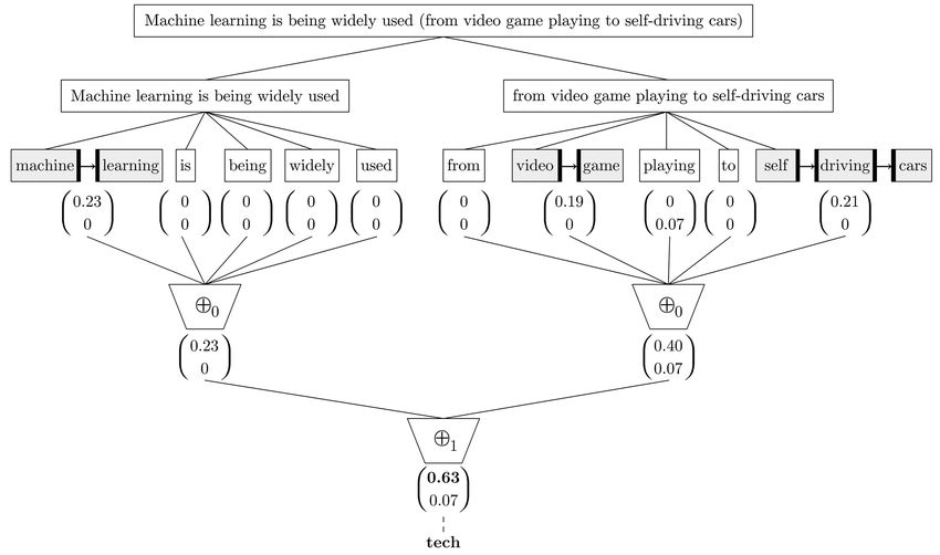
well-known in the standard document classification field, position corresponds to f ood, the second to music, and so
in which word n-grams are usually used to overcome them. on.
Unfortunately, when dealing with text streams, using word The computation of gv involves three functions, lv, sg
n-grams is not a trivial task since the system has to dy- and sn, as follows:
namically identify, create and learn which n-grams are
important “on the fly”. gv(w, c) = lvσ (w, c) · sgλ (w, c) · snρ (w, c) (1)
In this paper, we introduce a modification of SS3, called
τ -SS3, which expands its original definition to allow recog- • lvσ (w, c) values a word based on the local frequency of
nizing important word sequences. In Section 2 the original w in c. As part of this process, the word distribution
SS3 definition is briefly introduced. Section 3 formally curve is smoothed by a factor controlled by the hyper-
introduces τ -SS3, in which the needed equations and algo- parameter σ.
rithms are described. In Section 4 we evaluate our model
• sgλ (w, c) captures the global significance of w in c, it
on the CLEF’s eRisk 2017 and 2018 tasks on early depres-
decreases its value in relation to the lv value of w in
sion and anorexia detection. Finally, Section 5 summarizes
the other categories; the hyper-parameter λ controls
the main conclusions derived from this work.
how far the local value must deviate from the median
to be considered significant.
2. The SS3 Text Classifier
• snρ (w, c) sanctions lv in relation to how many other
As it is described in more detail in [1], SS3 first builds categories w is significant (sgλ (w, c) ≈ 1) to. That is,
a dictionary of words for each category during the training The more categories ci whose sgλ (w, ci ) is high, the
phase, in which the frequency of each word is stored. Then, smaller the snρ (w, c) value. The ρ hyper-parameter
using these word frequencies, and during the classification controls how sensitive this sanction is.
stage, it calculates a value for each word using a function
gv(w, c) to value words in relation to categories.1 gv takes To keep this paper shorter and simpler we will only
a word w and a category c and outputs a number in the introduce here the equation for lv since the computation of
interval [0,1] representing the degree of confidence with both, sg and sn, is based only on this function. Nonetheless,
which w is believed to exclusively belong to c, for instance, for those readers interested in knowing how sg and sn
suppose categories C = {f ood, music, health, sports}, we functions are actually computed, we highly recommend
could have: reading the SS3 original paper[1]. Thus, lv is defined as:
σ
P (w|c)
gv(‘sushi’, f ood) = 0.85; gv(‘the’, f ood) = 0; lvσ (w, c) = (2)
P (wmax |c)
gv(‘sushi’, music) = 0.09; gv(‘the’, music) = 0;
gv(‘sushi’, health) = 0.50; gv(‘the’, health) = 0;
gv(‘sushi’, sports) = 0.02; gv(‘the’, sports) = 0; Which, after estimating the probability, P , by analytical
Maximum Likelihood Estimation(MLE), leads to the actual
Additionally, a vectorial version of gv is defined as: definition:
−
→
gv(w) = (gv(w, c0 ), gv(w, c1 ), . . . , gv(w, ck ))
σ
tfw,c
where ci ∈ C (the set of all the categories). That is, −
→ is
gv lvσ (w, c) =
max{tfc }
(3)
only applied to a word and it outputs a vector in which
each component is the word’s gv for each category ci . For
instance, following the above example, we have: Where tfw,c denotes the frequency of w in c and max{tfc }
the maximum frequency seen in c. The value σ ∈ (0, 1] is
−
→
gv(‘sushi’) = (0.85, 0.09, 0.5, 0.02); one of the SS3’s hyper-parameter, called “smoothness”.
−
→
gv(‘the’) = (0, 0, 0, 0);
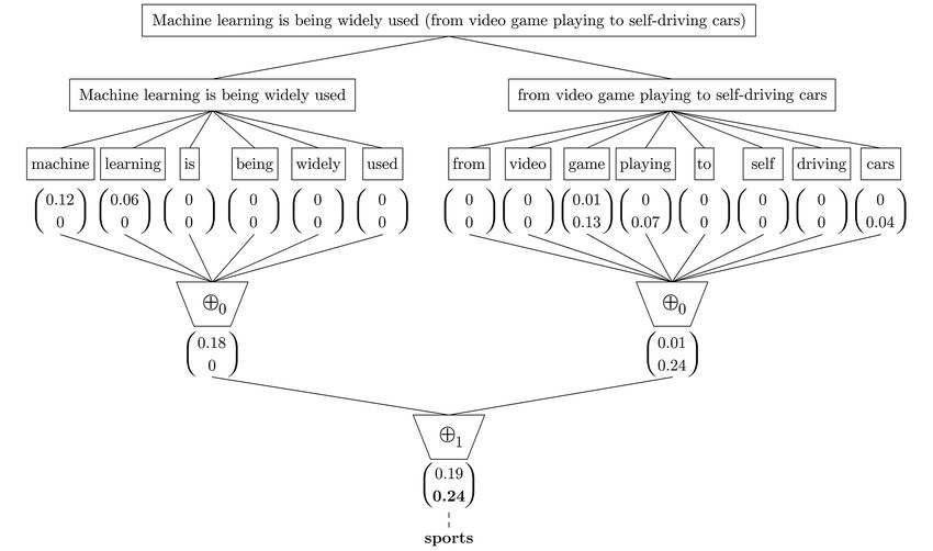
As it is illustrated in Figure 1, the SS3 classification
The vector −
→
gv(w) is called the “confidence vector of w”. algorithm can be thought of as a 2-phase process. In the
Note that each category is assigned a fixed position in − →
gv. first phase, the input is split into multiple blocks (e.g. para-
For instance, in the example above (0.85, 0.09, 0.5, 0.02) graphs), then each block is in turn repeatedly divided into
is the confidence vector of the word “sushi” and the first smaller units (e.g. sentences, words). Thus, the previously
“flat” document is transformed into a hierarchy of blocks.
In the second phase, the − → function is applied to each
gv
1 gv stands for “global value” of a word. In contrast with “local word to obtain the “level 0” confidence vectors, which then
value” (lv) which only values a word according to its frequency in a are reduced to “level 1” confidence vectors by means of
given category, gv takes into account its relative frequency across all a level 0 summary operator, ⊕0 . This reduction process
the categories.
is recursively propagated up to higher-level blocks, using
2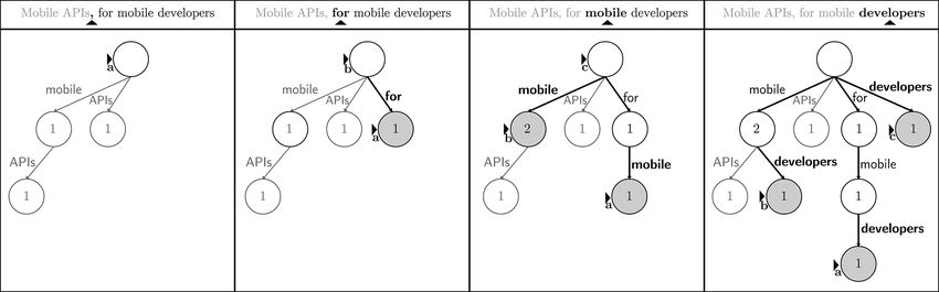
Figure 1: Classification example for categories technology and sports. In this example, SS3 misclassified the document’s topic as sports since it
failed to capture important sequences for technology like “machine learning” or “video game”. This was due to each sentence being processed
as a bag of words.

higher-level summary operators, ⊕j , until a single confi-                 when working with text streams, using n-grams is not triv-
               →
               −                                                           ial, since the system has to dynamically identify and learn
dence vector, d , is generated for the whole input. Finally,
the actual classification is performed based on the values                 which n-grams are important “on the fly”. In the next
                                  →
                                  −                                        section, we will introduce a variation of SS3, we have called
of this single confidence vector, d , using some policy —for
example, selecting the category with the highest confidence                τ -SS3, which expands the model definition to allow it to
value. Note that using the confidence vectors in this hi-                  dynamically recognize important word sequences.
erarchy of blocks, it is quite straightforward for SS3 to
visually justify the classification if different blocks of the             3. The τ -SS3 Text Classifier
input are colored in relation to their values. This is quite
relevant, especially when it comes to health-care systems,                     Regarding the model’s formal definition, the only change
specialists should be able to manually analyze the reasons                 we need to introduce is a generalized version of the lv func-
behind automatic users classifications.                                    tion given in Equation 2. This is trivial because it only in-
                                                                           volves allowing lv to value not only words but also sequences
    Note that SS3 processes individual sentences using a                   of them. That is, in symbols, if tk = w1 →w2 . . . →wk is a
bag-of-word model since the ⊕0 operators reduce the con-                   sequence of k words, then lv is now defined as:
fidence vectors of individual words into a single vector.                                                                    σ
                                                                                                        P (w1 w2 . . . wk |c)
Therefore, it is not being taken into account any relation-                            lvσ (tk , c) =                                (4)
ship that could exist between these individual words, for                                               P (m1 m2 . . . mk |c)
instance, between “machine” and “learning” or “video”
and “game”. That is, the model cannot capture impor-                           where m1 m2 . . . mk is the sequence of k words with the
tant word sequences that could improve the classification                  highest probability of occurring given that the category is
performance, as could have been possible in the example                    c.
shown in Figure 1. In addition, by allowing the model to                       Then, the same way as with Equation 3, the actual
capture important sequences, we also improve its ability                   definition of lv becomes:
to visually explain its rationale —for instance, think of                                                             σ
“self-driving cars” in relation to technology, this sequence                                                  tftk ,c
                                                                                            lvσ (tk , c) =                          (5)
could be highlighted and presented to the user instead of                                                    max tfk,c
each word being overlooked since none of “driving”, “cars”
and “self” are relevant to technology. In standard docu-
ment classification scenarios, this type of relationship could                Where tftk ,c denotes the frequency of sequence tk in
be captured using variable-length n-grams. Unfortunately,                  c and max{tfk,c } the maximum frequency seen in c for
                                                                           sequences of length k.

                                                                       3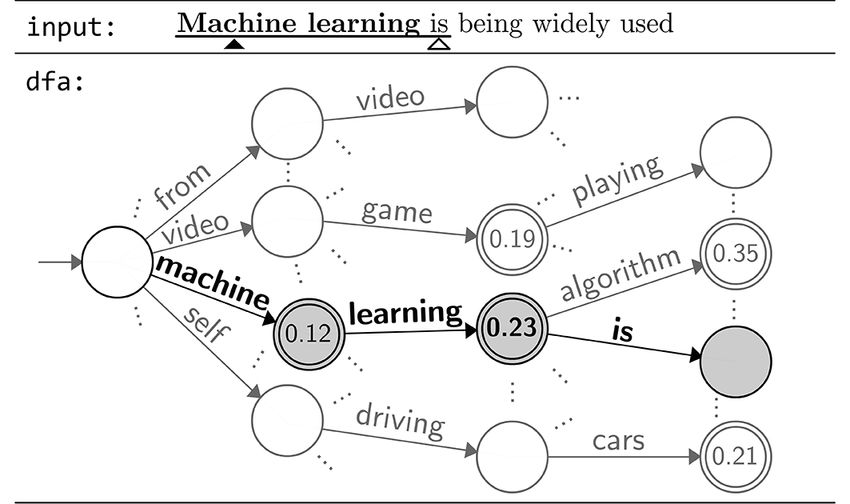
Figure 2: τ -SS3 classification example. Since SS3 now has the ability to capture important word sequences, it is able to correctly classify the
document’s topic as tech.

                                                                            the frequencies, as shown in Algorithm 1. Note that instead
   Thus, given any word sequence tk , now we could use                      of having k different dictionaries, one for each k-grams (e.g.
the original Equation 1 to compute its gv(tk , c). For in-                  one for words, one for bigrams, etc.) we have decided to
stance, suppose τ -SS3 has learned that the following word                  use a single prefix tree since all n-grams will share common
sequences have the gv value given below:                                    prefix with the shorter ones. Additionally, note that instead
                                                                            of processing the input document k times, again one for
     gv(machine→learning, tech) = 0.23;                                     each k-grams, we have decided to use multiple cursors to
     gv(video→game, tech) = 0.19;                                           be able to simultaneously store all sequences allowing the
     gv(self →driving→cars, tech) = 0.21;                                   input to be processed as a stream. Finally, note that lines
                                                                            8 and 9 of Algorithm 1 ensure that we are only taking
    Then, the previously misclassified example could now                    into account n-grams that make sense, i.e. those composed
be correctly classified as shown in Figure 2. In the following              only of words. All these previous observations, as well as
subsections, we will see how this formal expansion is in                    the algorithm intuition, are illustrated with an example
fact implemented in practice, i.e. how the training and                     in Figure 3. This example assumes that the training has
classification algorithms are implemented to store learned                  just begun for the first time and that the short sentence,
sequences and to, in fact, dynamically recognize sequences                 “Mobile APIs, for mobile developers”, is the first document
like those of this example during classification time.                      to be processed. Note that this tree will continue to grow,
                                                                            later, as more documents are consumed.
3.1. Training                                                                   Thus, each category will have a prefix tree storing infor-
    The original SS3 learning algorithm only needs a dic-                   mation linked to word sequences in which there is a tree’s
tionary of term-frequency pairs for each category. Each                     node for each learned k-gram. Note that in Algorithm 1
dictionary is updated as new documents are processed —i.e.                  there will never be more than M AX LV L cursors and
unseen terms are added and frequencies of already seen                      that the height of the trees will never grow higher than
terms are updated. Note that these frequencies are the only                 M AX LV L since nodes at level 1 store 1-grams, at level 2
elements we need to store since to compute lv(w, c) we only                 store 2-gram, and so on.
need to know w’s frequency in c, tfw,c (see Equation 3).                        Finally, it is worth mentioning that this learning algo-
    Likewise, τ -SS3 learning algorithm only needs to store                 rithm allows us to keep the original one’s virtues. Namely,
frequencies of all word sequences seen while processing                     the training is still incremental (i.e. it supports online
training documents. More precisely, given a fixed positive                  learning) since there is no need neither to store all docu-
integer n, it must store information about all word k-grams                 ments nor to re-train from scratch every time new training
seen during training, with 1 ≤ k ≤ n —i.e. single words,                    documents are available, instead, it is only necessary to
bigrams, trigrams, etc. To achieve this, the new learning                   update the already created trees. Additionally, there is still
algorithm uses a prefix tree (also called trie)[5, 3] to store all          no need to compute the document-term matrix because,

                                                                       4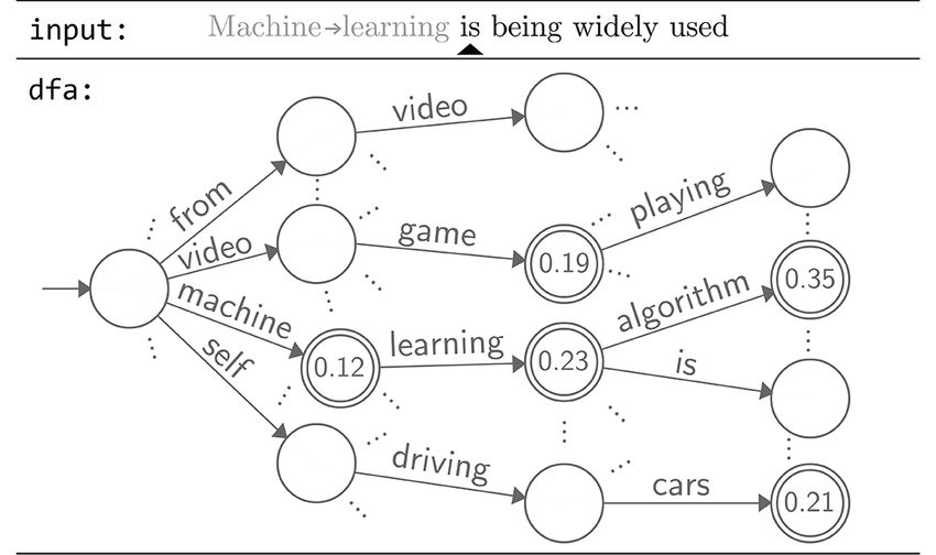
Figure 3: Training example. Gray color and bold indicate an update. (a) the first two words have been consumed and the tree has 3 nodes, one
for each word and one for the bigram “mobile APIs”, then a comma (,) is found in the input and Algorithm 1’s line 9 and 10 have removed all
the cursors and placed a new one, a, pointing to the root; (b) the word “for” is consumed, a new node for this word is created using the node
pointed by cursor a (lines 14), a is updated to point to this new node (line 15 and 20), the next term is read and a new cursor b is created (line
11) in the root; (c) “mobile” is consumed, using cursor b the node for this word updated its frequency to 2 (line 16), a new node is created for
the bigram “for mobile” using cursor a, and a new cursor c is created in the root node (line 11); (d) finally, the word “developers” is consumed
and similarly, new nodes are created for word “developers”, bigram “mobile developers” and trigram “for mobile developers”.

Algorithm 1 Learning Algorithm. Note that text is a se-                     sentences are split into single words, by allowing them to
quence of lexical units (terms) which includes not only words               be split into variable-length n-grams. Also, these n-grams
but also punctuation marks. M AX LV L stores the maximum                    must be “the best possible ones”, i.e. having the maximum
allowed sequence length.                                                    gv value. To achieve this goal, we will use the prefix tree
 1: procedure Learn-New-Document(text, category)                            of each category as a deterministic finite automaton (DFA)
 2:    input: text, a sequence of lexical units                             to recognize the most relevant sequences. Virtually, every
 3:            category, the category the document belongs to               node will we considered as a final state if its gv is greater
 4:    local variables: cursors, a set of prefix tree nodes                 or equal to a small constant . Thus, every DFA will
 5:                                                                         advance its input cursor until no valid transition could be
 6:    cursors ← an empty set                                               applied, then the state (node) with the highest gv value
 7:    for each term in text do                                             will be selected. This process is illustrated in more detail
 8:       if term is not a word then                                        in Figure 4.
 9:           cursors ← an empty set                                             Finally, the full algorithm is given in Algorithm 2.3 Note
10:       else
                                                                            that instead of splitting the sentences into words simply
11:           add category.Prefix-Tree.Root to cursors
12:           for each node in cursors do
                                                                            by using a delimiter, now we are calling a Parse function
13:              if node has not a child for term then                      on line 6. Parse intelligently splits the sentence into a
14:                  node.Child-Node.New(term)                              list of variable length n-grams. This is done by calling the
15:            child node ← node.Child-Node[term]                           Best-N-Gram function on line 20 which carries out the
16:            child node.Freq ← child node.Freq + 1                        process illustrated in Figure 4 to return the best n-gram
17:            if child node.Level ≥ M AX LV L then                         for a given category.
18:                remove node from cursors
19:            else
20:                replace node for child node in cursors
                                                                            4. Experimental Results
21: end procedure                                                           4.1. Datasets
                                                                                Experiments were conducted on the CLEF 2017[9] and
during classification and using Equation 5 and Equation 1,                  2018[10] eRisk open tasks, on early risk detection of depres-
gv could be dynamically computed based on the frequencies                   sion and anorexia. These pilot tasks focused on sequentially
stored in the trees.                                                        processing the content posted by users on Reddit. The

3.2. Classification                                                            3 Note that for this algorithm to be included as part of the SS3’s
    The original classification algorithm will remain mostly                overall classification algorithm, we only need to modify the original
unchanged2 , we only need to change the process by which                    definition of Classify-At-Level(text, n) of Algorithm 1 in [1] so
                                                                            that when called with n ≤ 1 it will call our new function, Classify-
      2 See
                                                                            Sentence.
              Algorithm 1 from [1].

                                                                        5
(a) (b)
Figure 4: Example of recognizing the best n-gram for the first sentence block of Figure 2, “Machine learning is being widely used”. For
simplicity in this example, we only show the technology’s DFA. There are conceptually 2 cursors, the black one (N) represents the input cursor
and the white one (M) the “lookahead” cursor to feed the automatons. (a) The lookahead cursor has advanced feeding the DFA with 3 words
(“machine”, “learning”, and “is”) until no more state transitions were available. There were two possible final states, one for “machine” and
another for “machine→ learning”, the latter is selected since it has the highest gv (0.23); (b) Finally, after the bigram “machine→ learning”
was recognized (see the first two word blocks painted in gray in Figure 2), the input cursor advanced 2 positions and is ready to start the
process again using “is” as the first word to feed the automatons.
datasets used in these tasks are a collection of writings (sub- 4.3. Results
missions) posted by users (referred to as “subjects”). The Results are shown in Table 1. As it can be seen, except
evaluation metric used in the eRisk tasks is called Early for ERDE5 in D18 and ERDE50 in A18, τ -SS3 outper-
Risk Detection Error (ERDE). The ERDE measure takes formed the best models. It is worth mentioning that, al-
into account not only the correctness of the system’s output though not included in the table, the new model improved
but also the delay taken to emit the decision. Additionally, the original SS3’s performance not only according to the
the ERDE measure is parameterized by a parameter, o, ERDE measures but also to most of the traditional/timeless
which serves as the “deadline” for decision making, i.e. if measures. For instance, in the eRisk 2017 early depression
a correct positive decision is made in time k > o,4 it will detection task, τ -SS3’s recall, precision and F1 were 0.55,
be taken by ERDEo as if it were incorrect (false positive). 0.43 and 0.77 respectively, against SS3’s 0.52, 0.44 and 0.63.
Finally, the performance of all participants was measured In addition, although these values were not the best among
using ERDE5 and ERDE50 . all participants, they were well above the average (0.39,
Due to space limitations, we are not introducing here the 0.36 and 0.51), which is not bad if we consider that hyper-
details about the datasets or the ERDE measure, however, parameter values of our model were selected to optimize
they can be found in [9] and [10]. the ERDE50 measure.
Results imply that learned n-grams contributed to im-
4.2. Implementation details proving the performance of our classifier. Furthermore,
The classifier was manually coded in Python 2.7 using these n-grams also improved the visual explanations given
only built-in functions and data structures (such as dict, by SS3, as illustrated in Figure 5.6
map and reduce functions, etc.). Source code is available
at https://github.com/sergioburdisso/ss3. Additionally,
to avoid wasting memory by letting the digital trees to 5. Conclusions
grow unnecessary large, every million words we executed a
In this article, we introduced τ -SS3, a novel text classi-
“pruning” procedure in which all the nodes with a frequency
fier that is able to learn and recognize useful patterns over
less or equal than 10 were removed. We also fixed the
text streams “on the fly”. We saw how τ -SS3 was defined
maximum n-gram length to 3 (i.e. we set M AX LV L =
as an expansion of the SS3 classifier. The new model uses
3).5 Finally, we used the same hyper-parameter values
a prefix tree to store variable-length n-grams seen during
as used in [1], namely we set λ = ρ = 1 and σ = 0.455.
training. The same data structure is then used as a DFA
The early classification policy we used was to classify test
to recognize important word sequences as the input is read.
subjects as positive as soon as the positive accumulated
confidence value exceeds the negative.
6 We have built an online live demo to try out τ -SS3, available at
4 Timeis measured in terms of user writings. http://tworld.io/ss3, in which along with the classification result it
5 Wetested other values greater than 3 but we did not notice any gives you interactive visual explanations similar to the one shown in
improvements on classification performance. this figure.
6Algorithm 2 Sentence classification algorithm. Map applies Table 1: Results on the eRisk tasks measured by ERDE (the lower, the
better). The tasks are “D17” and “D18” for Depression detection on
the gv function to every n-gram in ngrams and returns a list
eRisk 2017 and 2018 respectively, and “A18” for Anorexia detection
of resultant vectors. Reduce reduces ngrams cvs to a single on eRisk 2018. For comparison purposes, the models with the best
vector by applying the ⊕0 operator cumulatively. ERDE5 and ERDE50 in the competitions are also included.
1: function Classify-Sentence(sentence) returns a confi-
Task Model ERDE5 ERDE50
dence vector
τ -SS3 12.6% 7.70%
2: input: sentence, a sequence of lexical units D17
3: local variables: ngrams, a sequence of n-grams SS3 12.6% 8.12%
4: ngrams cvs, confidence vectors UNSLA 13.66% 9.68%
5: FHDO-BCSGB 12.70% 10.39%
6: ngrams ← Parse(sentence) τ -SS3 9.48% 6.17%
D18
7: ngrams cvs ← Map(gv, ngrams) SS3 9.54% 6.35%
8: return Reduce(⊕0 , ngrams cvs) UNSLA 8.78% 7.39%
9: end function FHDO-BCSGA 9.50% 6.44%
τ -SS3 11.31% 6.26%
10: function Parse(sentence) returns a sequence of n-grams A18
SS3 11.56% 6.69%
11: input: sentence, a sequence of lexical units
FHDO-BCSGD 12.15% 5.96%
12: global variables: categories, the learned categories
13: local variables: ngram, a sequence of words UNSLB 11.40% 7.82%
14: output, a sequence of n-grams
15: bests, a list of n-grams
16:
17: cur ← the first term in sentence
18: while cur is not empty do
19: for each cat in categories do (a) Sentence level
20: bests[cat] ← Best-N-Gram(cat, cur)
21: ngram ← the n-gram with the highest gv in bests
22: add ngram to output
23: move cur forward ngram.Length positions
24: return output (b) Word level
25: end function
Figure 5: This figure shows the visual description given in Figure 9
26: function Best-N-Gram(cat, term) returns a n-gram of [1]. It shows the subject 9579’s writing 60 of the 2017 depression
27: input: cat, a category detection task. The visual description is shown at different levels: (a)
28: term, a cursor pointing to a term in the sentence sentences and (b) words. Blocks are painted proportionally to the
real confidence values we obtained for the depression category after
29: local variables: state, a node of cat.Prefix-Tree
experimentation. Note that more useful information is now shown,
30: ngram, a sequence of words such as the n-grams “I was feeling” and “kill myself”, improving the
31: best ngram, a sequence of words richness of visual explanations.
32:
33: state ← cat.Prefix-Tree.Root
34: add term to ngram References
35: best ngram ← ngram
36: while state has a child for term do [1] Burdisso, S.G., Errecalde, M., y Gómez, M.M.: A text
37: state ← state.Child-Node[term] classification framework for simple and effective early
depression detection over social media streams. Ex-
38: term ← next word in the sentence
pert Systems with Applications 133, 182 – 197 (2019).
39: add term to ngram https://doi.org/10.1016/j.eswa.2019.05.023, http://www.
40: if gv(ngram, cat) > gv(best ngram, cat) then sciencedirect.com/science/article/pii/S0957417419303525
41: best ngram ← ngram [2] Burdisso, S.G., Errecalde, M., y Gómez, M.M.: UNSL at erisk
42: return best ngram 2019: a unified approach for anorexia, self-harm and depression
detection in social media. In: Experimental IR Meets Multi-
43: end function
linguality, Multimodality, and Interaction. 10th International
Conference of the CLEF Association, CLEF 2019. Springer In-
ternational Publishing, Lugano, Switzerland (2019)
This allowed us to keep all the original SS3’s virtues: sup- [3] Crochemore, M., Lecroq, T.: Trie. Encyclopedia of Database
port for incremental classification and learning over text Systems pp. 3179–3182 (2009)
[4] Escalante, H.J., Villatoro-Tello, E., Garza, S.E., López-Monroy,
streams; easy support for early classification; and visual A.P., Montes-y Gómez, M., Villaseñor-Pineda, L.: Early detec-
explainability. τ -SS3 showed an improvement over the orig- tion of deception and aggressiveness using profile-based repre-
inal SS3 in terms of standard performance metrics as well sentations. Expert Systems with Applications 89, 99–111 (2017)
as for ERDE metrics. It also showed an improvement in [5] Fredkin, E.: Trie memory. Communications of the ACM 3(9),
490–499 (1960)
terms of the expressiveness of visual explanations. [6] Iskandar, B.S.: Terrorism detection based on sentiment analysis
7using machine learning. Journal of Engineering and Applied
Sciences 12(3), 691–698 (2017)
[7] Kwon, S., Cha, M., Jung, K.: Rumor detection over varying
time windows. PloS one 12(1), e0168344 (2017)
[8] Losada, D.E., Crestani, F.: A test collection for research on
depression and language use. In: International Conference of the
Cross-Language Evaluation Forum for European Languages. pp.
28–39. Springer (2016)
[9] Losada, D.E., Crestani, F., Parapar, J.: erisk 2017: Clef lab on
early risk prediction on the internet: Experimental foundations.
In: International Conference of the Cross-Language Evaluation
Forum for European Languages. pp. 346–360. Springer (2017)
[10] Losada, D.E., Crestani, F., Parapar, J.: Overview of erisk: early
risk prediction on the internet. In: International Conference of
the Cross-Language Evaluation Forum for European Languages.
pp. 343–361. Springer (2018)
[11] Ma, J., Gao, W., Mitra, P., Kwon, S., Jansen, B.J., Wong, K.F.,
Cha, M.: Detecting rumors from microblogs with recurrent
neural networks. In: IJCAI. pp. 3818–3824 (2016)
[12] Ma, J., Gao, W., Wei, Z., Lu, Y., Wong, K.F.: Detect rumors
using time series of social context information on microblogging
websites. In: Proceedings of the 24th ACM International on
Conference on Information and Knowledge Management. pp.
1751–1754. ACM (2015)
8You can also read