INTRODUCTION TO DEEP LEARNING - (AND MATERIALS SCIENCE APPLICATIONS) - PART 2 - NOMAD COE

Introduction to
Deep Learning
(and Materials Science
applications) – part 2

1 2 3 4
 Part 1. Part 2. Part 3. Part 4.
 Recurrent Neural Long Short Term Memory Generative Adversarial Miscellaneous
 Networks (RNNs) (LSTM) Networks (GANs)

 Lecture 2 Outline

INTRODUCTION TO DEEP LEARNING // ANGELO ZILETTI, PHD // JANUARY 2021 2

Main references for this class
  Dive into Deep Learning (https://d2l.ai/)
  Authors: Aston Zhang and Zachary C. Lipton and Mu Li and Alexander J. Smola
  Interactive deep learning book with code, math, and discussions
  Implemented with NumPy/MXNet, PyTorch, and TensorFlow
  Adopted at 140 universities from 35 countries

  Deep Learning, MIT Press Book (https://www.deeplearningbook.org/)
  Authors: Ian Goodfellow and Yoshua Bengio and Aaron Courville

  Introduction to Deep Learning (MIT online course) http://introtodeeplearning.com/
  Authors: A. Amini, and A. Soleimany

INTRODUCTION TO DEEP LEARNING // ANGELO ZILETTI, PHD // JANUARY 2021 3

1 2 3 4
 Part 1. Part 2. Part 3. Part 4.
 Recurrent Neural Long Short Term Memory Generative Adversarial Miscellaneous
 Networks (RNNs) (LSTM) Networks (GANs)

 Lecture 2 Outline

INTRODUCTION TO DEEP LEARNING // ANGELO ZILETTI, PHD // JANUARY 2021 4

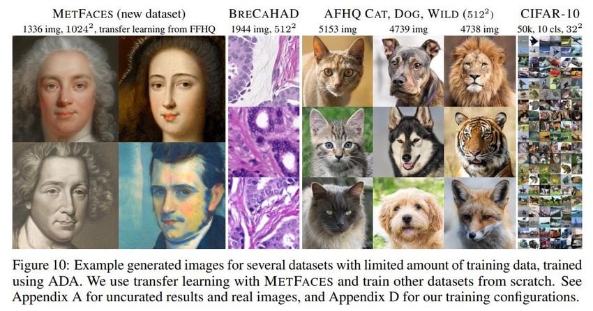
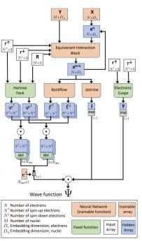
When the order of the data matters
  So far we encountered two types of data:
  tabular data (multi-layer perceptron or MLP)
  grid-like data (convolutional neural networks or CNN) – specialized architecture

  Collected observation pairs ( ⅈ
 , ⅈ ) with one key assumption: the order of the data does not matter
 (examples are independent and identically distributed, i.i.d.)
  … but what about sequences? They are not i.i.d. by definition

 ෡ 
 
 min = min =
 2

 Hermann et al., Nat. Chem. 12, 891 (2020)
 Pfau et al., Phys. Rev. Research 2, 033429 (2020) M. Ziatdinov et al., ACS nano 11, 12742 (2017) A. Ziletti et al., Nature Communications, 9, 2775 (2018)

INTRODUCTION TO DEEP LEARNING // ANGELO ZILETTI, PHD // JANUARY 2021 5

Predictions based on sequences
  Some applications:
  Speech recognition
  Music generation
  Sentiment classification of text
  Machine Translation
  DNA sequence analysis

  In physics/materials science:
  Any ideas?
  Treat experimental spectra or in general any temporal signal
  Molecular properties (molecule seen as a sequence)

INTRODUCTION TO DEEP LEARNING // ANGELO ZILETTI, PHD // JANUARY 2021 6

Sequence model
  Example: predict stock prices (as quantified by the S&P 500 index)
  is the index value at time step ; discrete
  Prediction on day (= time step) :
 ො = ȁ −1 , … , 1

  Prediction of the future in principle depends on the past
  This dependency on the past is a major problem:
  the number of inputs −1 , … , 1 varies, depending on 
 (A proxy for) stock prices: S&P 500 index in 2020
  Complexity increases with the amount of data that we encounter
  Approximations needed to make ȁ −1 , … , 1 computationally
 tractable
  The goal of sequence modelling is to find good approximations (like we did
 with CNN previously)

INTRODUCTION TO DEEP LEARNING // ANGELO ZILETTI, PHD // JANUARY 2021 7

Autoregressive models
  We need to approximate ȁ −1 , … , 1

  Autoregressive models:
  Assumes that the entire sequence −1 , … , 1 is actually not necessary
  Keep only some timespan of length , only use −1 , … , − (if = 1: first-order Markov process)

  Number of arguments is fixed: one can train a deep network as seen before (e.g. MLP)
  These models perform regression on themselves (hence the name) (e.g. auto-regressive moving average (ARMA) models)
  Some questions:
  How to chose the right ? Is there even a right ?
  Sometimes we need to look far away in the past, sometimes not

  Wouldn’t it be better to look at the whole sequence and keep only relevant information from the past?

INTRODUCTION TO DEEP LEARNING // ANGELO ZILETTI, PHD // JANUARY 2021 8

Latent autoregressive models
  Introduce a latent state ℎ 
 ො −1 ො ො +1
  ℎ summarizes all the relevant information about the past
  At every new timestep, update the latent state ℎ state as
 follows:
 ℎ −1 ℎ ℎ +1
 ℎ = ℎ −1 , 
  This exploit the fact that ℎ −1 summarizes the past up to − 1; it is a
 recurrent relation
 −2 −1 
  The prediction ො is thus approximated by
 ො = ȁ −1 , … , 1 ≈ ȁℎ 

  Arbitrary length sequence −1 , … , 1 mapped to a fixed length vector ℎ → ℎ is a lossy summary of the past
  Recurrent neural networks (RNNs) aim at learning this (crucial) mapping function from data

INTRODUCTION TO DEEP LEARNING // ANGELO ZILETTI, PHD // JANUARY 2021 9

Recurrent Neural Network (RNN)
  When trained to perform a task that requires predicting the
 future from the past, the RNN learns to use ℎ as a lossy
 yො Output vector summary of the task-relevant aspects of the past
 sequence of inputs (up to )
  Do this by applying a recurrence relation at every time step
 to process a sequence:
 ℎ = ℎ −1 , 
 RNN  ℎ : cell state
 recurrent cell ℎ  : mapping function parameterized by 
  ℎ −1 : old state
  : input vector at time step 
  This mapping function is fixed
 Input vector  assumption: the dynamics of the sequence itself does not
 change (stationary)

INTRODUCTION TO DEEP LEARNING // ANGELO ZILETTI, PHD // JANUARY 2021 10

RNN state update and output

 Output Vector
 yො Output vector
 yො = ℎ ℎ + 

 RNN Update Hidden State:
 recurrent cell ℎ ℎ = σ( ℎℎ ℎ −1 + ℎ + ℎ )

 Input vector Input vector:
 
INTRODUCTION TO DEEP LEARNING // ANGELO ZILETTI, PHD // JANUARY 2021 11

MLP, and RNN modelling for sequence data

 yො

 Other
 architectures
 are possible

 Many to One Many to Many
 One to One Sentiment Classification Machine Translation – Text generation
“Vanilla” neural network Spectrum to property
 (e.g. MLP)

INTRODUCTION TO DEEP LEARNING // ANGELO ZILETTI, PHD // JANUARY 2021 12

Unfolding the RNN: computational graph across time

 Forward pass 
 0 1 2 

 yො yො 0 yො1 yො 2 … yො T

 ℎ ℎ ℎ ℎ

 RNN = ℎℎ ℎℎ ℎℎ
 …
 ℎ ℎ ℎ ℎ 

 0 1 2 … 

 The same weight matrices are re-used at every step
 Assumption: the dynamics of the sequence itself does not change (stationary)
INTRODUCTION TO DEEP LEARNING // ANGELO ZILETTI, PHD // JANUARY 2021 13

RNN: backpropagation trough time

 Forward pass 
 0 1 2 
 Backward pass

 yො yො 0 yො1 yො 2 … yො T

 ℎ ℎ ℎ ℎ

 RNN = ℎℎ ℎℎ ℎℎ
 …
 ℎ ℎ ℎ ℎ 

 0 1 2 … 

INTRODUCTION TO DEEP LEARNING // ANGELO ZILETTI, PHD // JANUARY 2021 14

Standard RNN gradient flow: some considerations
  The loss function depends on the errors at all time steps: 
 0 1 2 
 1
 = ෍ ො , 
 
 =1
 yො 0 yො1 yො 2
 … yො T
  To train the network, we need to calculate the gradients ℎ ℎ ℎ ℎ
 
 ℎ 
 and 
 ℎℎ
 of the loss function w.r.t. the network
 ℎℎ ℎℎ ℎℎ …
 parameters ℎℎ and ℎ ℎ ℎ ℎ ℎ 

  We have done the same for MLPs in the previous lecture 0 1 2 … 

  However, in RNN is more complicated because ℎ depends recursively on hidden states at all previous
 timesteps through the recurrent relation
 = ℎ −1 , or equivalently = σ( ℎℎ −1 + ℎ + ℎ )
  Repeated application of the chain rule

INTRODUCTION TO DEEP LEARNING // ANGELO ZILETTI, PHD // JANUARY 2021 15

Standard RNN gradient flow: vanishing and exploding gradients
  It can be shown (neglecting biases and activation function in the hidden layer being the identity) [1] :
 
 ⊤
  =෍ prod , =෍ 
 ℎ =1 ℎ =1 

 ⊤
  =෍ prod , =෍ −1
 ℎℎ =1 ℎℎ =1 

 where the central quantity (affecting numerical stability) is :
 
 −1 
 = ෎ ⊤
 ℎℎ ⊤
 yh
 ෝ
 + −ⅈ
 =1

 involves large powers of ⊤
 
 
 ℎℎ for long sequence models (scales as the # of input steps )

  This leads to the so-called “exploding and vanishing gradient problem” in standard RNN

 [1] 8.7. Backpropagation Through Time — Dive into Deep Learning 0.15.1 documentation (d2l.ai)
INTRODUCTION TO DEEP LEARNING // ANGELO ZILETTI, PHD // JANUARY 2021 16

Standard RNN gradient flow: vanishing and exploding gradients

 ℎ0 ℎ1 ℎ2 ℎ 
 ℎℎ ℎℎ ℎℎ −1 
 ℎ ℎ ℎ ℎ = ෎ ⊤
 ℎℎ ⊤
 yh
 ෝ
 + −ⅈ
 0 1 2 … =1

  Computing the gradient involves many factors of ℎℎ and a repeated gradient computation
 0

 Many (eigen)values of ℎℎ > 1: Many (eigen)values of ℎℎ < 1:
 exploding gradients vanishing gradients

 Solution (easy): Solution (hard):
 Gradient clipping to scale large gradients Some heuristics (activation functions, weight initialization)
 Specialized network architectures

INTRODUCTION TO DEEP LEARNING // ANGELO ZILETTI, PHD // JANUARY 2021 17

The need for specialized neural network architectures for sequences
  Observation 1: Long sequences are needed to accomplish most tasks:
  Bob and Alice are going out for a walk. Bob picks and gives _____ a flower.

  My name is Paul, I am German, currently living in Florence. I love the food and the people, but I really miss speaking ______ .

  Observation II: not all observations in a sequence are equally relevant

  Main idea to accomplish that: build-in mechanisms in the RNN to remember only relevant
 observations
  Mechanism to pay attention (i.e. Is the input at the current timestep relevant for the task?) – Input gate
  Mechanism to forget (i.e. Is some past information now irrelevant for the task?) – Forget gate
  Mechanism to easily carry over the information to the next steps – Memory Cell (cell state)
  This is accomplished through specialized architectures for sequences: most popular are LSTM or GRU

INTRODUCTION TO DEEP LEARNING // ANGELO ZILETTI, PHD // JANUARY 2021 18

1 2 3 4
 Part 1. Part 2. Part 3. Part 4.
 Recurrent Neural Long Short Term Memory Generative Adversarial Miscellaneous
 Networks (RNNs) (LSTM) Networks (GANs)

 Lecture 2 Outline

INTRODUCTION TO DEEP LEARNING // ANGELO ZILETTI, PHD // JANUARY 2021 19

Simple RNN: one simple layer
  The repeating module in a standard RNN contains a single layer:

[LSTM paper] Hochreiter and Schmidhuber, Neural Computation 9(8):1735, (1997)
Figure from d2l.ai (https://d2l.ai/chapter_recurrent-neural-networks/rnn.html
INTRODUCTION TO DEEP LEARNING // ANGELO ZILETTI, PHD // JANUARY 2021 20

Long Short Term Memory (LSTM): four interacting layers instead of one
  The repeating module in an LSTM contains four interacting layers:

[LSTM paper] Hochreiter and Schmidhuber, Neural Computation 9(8):1735, (1997)
Figure from d2l.ai (https://d2l.ai/chapter_recurrent-neural-networks/rnn.html)
INTRODUCTION TO DEEP LEARNING // ANGELO ZILETTI, PHD // JANUARY 2021 21

The Core Idea Behind LSTMs: gated memory cell

  LSTM’s design is inspired by logic gates of a computer
  LSTM introduces a memory cell (or cell for short) that has the
 same shape as the hidden state engineered to record additional
 information.
  This allows to information to easily flow from one step to the
 next

  Information is added or removed through structures called gates
  Gates are composed by a sigmoid neural net layer and a pointwise
 multiplication operation
  The sigmoid layer outputs numbers between zero and one, describing how
 much of each component should be let through

 Figures from d2l.ai (https://d2l.ai/chapter_recurrent-neural-networks/rnn.html)
INTRODUCTION TO DEEP LEARNING // ANGELO ZILETTI, PHD // JANUARY 2021 22

LSTM: remembering what is important through memory cell and gates

  Different gates control the memory cell
  Forget gate: mechanism to reset the content of the cell
  Input gate: decides when to read data into the cell.
  Output gate: reads out the entries from the cell

  Motivation: to be able to decide when to remember
 and when to ignore inputs in the hidden state via a
 dedicated mechanism
  Implements the main idea (discussed before) for
 sequence learning: build-in mechanisms in to remember
 only relevant observations

From d2l.ai (https://d2l.ai/chapter_recurrent-neural-networks/rnn.html)
INTRODUCTION TO DEEP LEARNING // ANGELO ZILETTI, PHD // JANUARY 2021 23

Input gate, forget gate, output gate
  Data feeding into the LSTM gates are
  input at the current time step 
  hidden state of the previous time step −1
  Data processed by three fully-connected layers with a sigmoid
 activation function to compute the values of the input, forget and
 output gates:
  = σ( ⅈ + ⅈℎ −1 + ⅈ )
  = σ( + ℎ −1 + )
  = σ( + ℎ −1 + )
 where ⅈ , , , ⅈℎ , ℎ , ℎ are weight parameters and ⅈ , , and
 are bias parameters
  As a result of the sigmoid activation, values of the three gates are in the
 range of (0,1)

From d2l.ai (https://d2l.ai/chapter_recurrent-neural-networks/rnn.html)
INTRODUCTION TO DEEP LEARNING // ANGELO ZILETTI, PHD // JANUARY 2021 24

Candidate memory cell
  We introduce the candidate memory cell
  It builds the candidate update for the memory cell

  It is a fully-connected layer (like the other gates), but using
 a tanh function instead:
 ෤ = tanh + ℎ −1 + 

 where , ℎ are weight parameters and is a bias parameter

  ෤ is in the range for (−1,1) as the activation function.

From d2l.ai (https://d2l.ai/chapter_recurrent-neural-networks/rnn.html)
INTRODUCTION TO DEEP LEARNING // ANGELO ZILETTI, PHD // JANUARY 2021 25

Memory cell update
  We need a mechanism to govern input and forgetting
  Two gates for this:
  Input gate : decides how much we take data into account via the
 candidate cell ෤ 
  Forget gate : decides how much of the old memory cell content
 we keep
  Update equation for the memory cell:
 = ⊙ −1 + ⊙ ෤ 
 where ⊙ indicates elementwise multiplication

  If gate is always approximately 1 and the is always approximately 0, the past memory cells −1 will be saved
 over time and passed to the current time step (no reliance on gradients)
  alleviates the vanishing gradient problem and to better capture long range dependencies within sequences

From d2l.ai (https://d2l.ai/chapter_recurrent-neural-networks/rnn.html)
INTRODUCTION TO DEEP LEARNING // ANGELO ZILETTI, PHD // JANUARY 2021 26

Hidden state update
  We need compute the update of the hidden state 
  In LSTM, the hidden state is simply a gated version of the
 tanh memory cell
  Output gate : decides how much data will be copied
 from the memory cell to the hidden state 
  Update equation for hidden state :
 = ⊙ tanh( )
 where ⊙ indicates elementwise multiplication

  If approximates 1: pass all memory information through to the predictor
  If approximates 0: retain all the information only within the memory cell

INTRODUCTION TO DEEP LEARNING // ANGELO ZILETTI, PHD // JANUARY 2021 27

LSTM applications
  LSTM have been tremendously successful in modelling long-term dependencies in sequences
  Examples of tasks performed with LSTM:
  Time-series prediction
  Speech recognition
  Handwritten recognition
  Sentiment classification (does this text has a positive, negative, or neural sentiment?)
  Machine translation
  Music generation
  Robot control
  Trajectory prediction in self driving cars

From Wikipedia (https://en.wikipedia.org/wiki/Long_short-term_memory)
INTRODUCTION TO DEEP LEARNING // ANGELO ZILETTI, PHD // JANUARY 2021 28

LSTM real-world applications
  LSTM has numerous applications in the real world [*]
  2015:
  Google started using an LSTM for speech recognition on Google Voice. According to the official blog post, the new model cut
 transcription errors by 49%.

  2016:
  Google released the Google Neural Machine Translation system for Google Translate which used LSTMs to reduce translation errors by
 60%.
  Apple announced in its Worldwide Developers Conference that it would start using the LSTM for quicktypein the iPhone and for Siri.
  Amazon released Polly, which generates the voices behind Alexa, using a bidirectional LSTM for the text-to-speech technology.

  2017: Facebook performed some 4.5 billion automatic translations every day using long short-term memory networks

  Currently the new state-of-the-art systems for sequence modellings are attention-based systems
  Key publication:Vaswani et al., Attention Is All You Need, ArXiv:1706.03762 (2017)

[*] From Wikipedia (https://en.wikipedia.org/wiki/Long_short-term_memory)
INTRODUCTION TO DEEP LEARNING // ANGELO ZILETTI, PHD // JANUARY 2021 29

Deep RNN
  So far, only a single layer architecture,
  We can however add more layers to make the model more flexible
 (and powerful)
  flexible because it allows to extract information at different levels
  Examples:
  Financial data: high-level data about financial market conditions (bear or bull
 market) available lower level: only record shorter-term temporal dynamics.
  Physics: high-level data about general behavior described by an effective theory;
 low-level: deviations from the effective theory due to interactions

  Deep simply means adding more layers
  Stack multiple layers of RNNs on top of each other.
  Each hidden state is continuously passed to both the next time step of the
 current layer and the current time step of the next layer Deep RNN with hidden layers.

Figure from d2l.ai (https://d2l.ai/chapter_recurrent-modern/deep-rnn.html)
INTRODUCTION TO DEEP LEARNING // ANGELO ZILETTI, PHD // JANUARY 2021 30

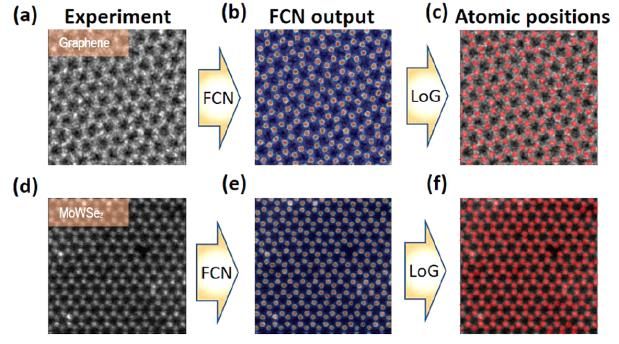
Revealing ferroelectric switching character using deep recurrent neural networks [1]
  Band-excitation piezoresponse (BEPS) force microscopy is
 used to characterize the nanoscale-switching processes (a
 variant of atomic force microscopy)
  Raw data is high-dimensional (amplitude, phase, resonance
 frequency, and quality factor of the cantilever resonance) and are
 are qualitative measures of piezoresponse, polarization direction,
 stiffness, and dampening
  Information of physical significance lies on a data manifold
 with a much lower dimensionality; however, no means to
 predict the manifold
  LSTM autoencoder can be used to learn characteristic
 mechanisms of response from multichannel hyperspectral BEPS
  This new capability provides a process to quantify subtle
 differences in switching mechanisms

[1] Agar et al., Nature Comm. 10, 4809 (2019)
INTRODUCTION TO DEEP LEARNING // ANGELO ZILETTI, PHD // JANUARY 2021 31

1 2 3 4
 Part 1. Part 2. Part 3. Part 4.
 Recurrent Neural Long Short Term Memory Generative Adversarial Miscellaneous
 Networks (RNNs) (LSTM) Networks (GANs)

 Lecture 2 Outline

INTRODUCTION TO DEEP LEARNING // ANGELO ZILETTI, PHD // JANUARY 2021 33

Generative vs Discriminative algorithms
  Discriminative algorithms: given the input features ⅈ , how likely are ⅈ ?
  They make predictions based on input data P ⅈ ห ⅈ

 ⅈ
  Given the features of a data instance , they predict a label (classification) or value (regression)
  Example 1: given all the words in an email (features), a discriminative algorithm could predict whether the message is spam or not spam
 (classification task)
  Example II: given the chemical composition and atomic position (features), a discriminative algorithm could predict the superconducting
 temperature (regression task)

  Generative algorithms: given ⅈ , how likely are the input features ⅈ ?
  Instead of predicting a label given certain features, they attempt to predict features given a certain label P ⅈ ห ⅈ

  Example I: assuming this email is spam, how likely are these words?
  Example II: given superconductive temperature = 250 , how likely are these chemical compositions and atomic positions? Or
 better, which chemical compositions and atomic positions are likely to give raise to a = 250 

  Given such a model, one could sample synthetic data that resemble the distribution of the training data

INTRODUCTION TO DEEP LEARNING // ANGELO ZILETTI, PHD // JANUARY 2021 34

Generative adversarial networks (GANs): intuition
  Generative Adversarial Networks (GANs) are a way to make a generative model by having two neural
 networks compete with each other

 Discriminator :
 tries to identify real date
 from the fakes created by
 Generator :
 (real data) the generator
 turns noise (random
 vector) into an
 imitation of the data to ො
 try to trick the
 
 discriminator

 ( )
 (fake data)

From Introduction to Deep Learning (MIT online course) http://introtodeeplearning.com/
INTRODUCTION TO DEEP LEARNING // ANGELO ZILETTI, PHD // JANUARY 2021 35

GAN minimax formulation
  Discriminator:
 
  a binary classifier to distinguish if the input is real (from real data, = 1) or fake (from the (real
 generator, =0) data)
 
  Goal: close to 1 (real data), ( ) close to 0 (fake data)
 ( )
  train the discriminator to minimize the cross-entropy for classifying real vs fake: (fake
 
 max = max ~ log + log(1 − ( )) data)
 
 where ~ denotes sampling from the training set
  Generator:
  Wants to fool the discriminator in classifying fake data in being real; ( close to 1
  min = min ~ log + ~ ⅈ log(1 − ( ))
 
  Discriminator and generator are playing a zero-sum game against each other:
 min max = min max ~ log + ~ ⅈ log(1 − ( ))
 
 Zero-sum game: a situation in which each participant's gain or loss is exactly balanced by the losses or gains of the other participants.

INTRODUCTION TO DEEP LEARNING // ANGELO ZILETTI, PHD // JANUARY 2021 36

GAN: generating realistic samples

Karras et al., NIPS 2020, ArXiv: 2006.06676

INTRODUCTION TO DEEP LEARNING // ANGELO ZILETTI, PHD // JANUARY 2021 37

1 2 3 4
 Part 1. Part 2. Part 3. Part 4.
 Recurrent Neural Long Short Term Memory Generative Adversarial Miscellaneous
 Networks (RNNs) (LSTM) Networks (GANs)

 Lecture 2 Outline

INTRODUCTION TO DEEP LEARNING // ANGELO ZILETTI, PHD // JANUARY 2021 38

Neural Networks for symbolic regression: AI-Feynman 2.0
  Symbolic Regression: [1]
  type of regression analysis that searches the space of mathematical expressions to find the model that best fits a given
 dataset, both in terms of accuracy and simplicity
  No particular model is provided as a starting point to the algorithm
  Initial expressions are formed by randomly combining mathematical building blocks such as mathematical
 operators, analytic functions, constants, and state variables.
  Symbolic regression using neural networks: AI Feynman 2.0 [2]
  Videotime: NeurIPS 2020 : AI Feynman 2.0: Pareto-optimal symbolic regression exploiting graph modularity

  Seeks to fit data to formulas that are Pareto-optimal, in the sense of having the best accuracy for a given complexity
  discovers generalized symmetries from gradient properties of a neural network fit
  uses a fully-connected, feed-forward neural network with 4 hidden layers of 128, 128, 64 and 64 neurons, respectively

[1] From Wikipedia [2] Udrescu et al., NIPS 2020, ArXiv: 2006.10782 [2]
INTRODUCTION TO DEEP LEARNING // ANGELO ZILETTI, PHD // JANUARY 2021 39

Interpretability in deep learning (and machine learning in general)
  Deep learning models are generally hard to interpret due to their complexity (distributed knowledge
 across millions of parameters)

  Despite that, there are methods that aim at interpreting neural networks
  A great resource on machine learning interpretability: C. Molnar, Interpretable Machine Learning,
 https://christophm.github.io/interpretable-ml-book/ Ludwig Maximilian University of Munich
  A review on neural network interpretability: Fan et al., ArXiv: 2001.02522 (2020)

  We will briefly discuss one of the most successful interpretation method: SHAP [1]
  SHAP unifies numerous available interpretation methods, including:
  LIME: Ribeiro et al., SIGKDD International Conference on Knowledge Discovery and Data Mining (2016)
  DeepLIFT: Shrikumar et al., arXiv preprint arXiv:1704.02685 (2017).
  Layer-wise relevance propagation: Bach al., PloS one 10.7 (2015)

[1] Lundberg and Lee, NIPS 2017, ArXiv: 1705.07874
INTRODUCTION TO DEEP LEARNING // ANGELO ZILETTI, PHD // JANUARY 2021 40

SHAP (SHapley Additive exPlanations)
  SHAP (SHapley Additive exPlanations): a game theoretic approach to explain the output of any machine
 learning model. [1]

  Main idea: Shapley value [2] calculate the importance of a feature by comparing what a model predicts with
 and without the feature
  Coalition of players cooperates, and obtains a certain overall goal
  Some players may contribute more to the coalition than others or may posses different bargain power
  Shapley value answers the question: How important is each player to the overall cooperation, and what payoff can
 each play reasonable expect?
  Machine learning application [1]:
  Overall gain → prediction
  Player importance → feature importance

[SHAP] [1] Lundberg and Lee, NIPS 2017, ArXiv: 1705.07874 [Shapley Value] [2] S. Shapley, Annals of Math. Studies, 28, 307 (1953)
INTRODUCTION TO DEEP LEARNING // ANGELO ZILETTI, PHD // JANUARY 2021 41

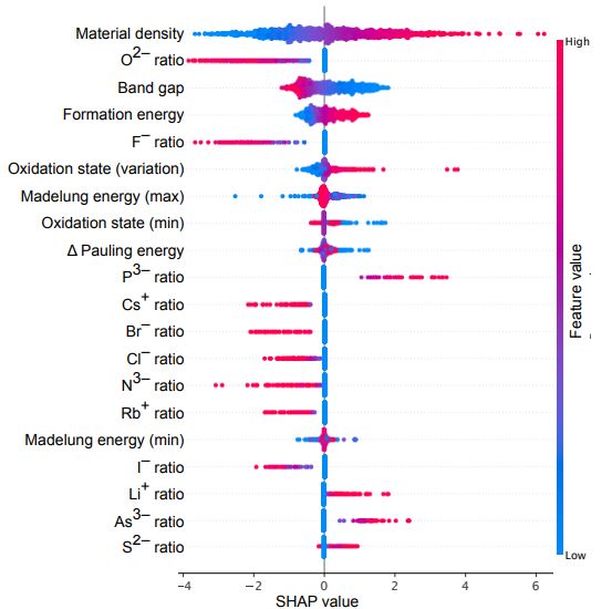
An example of SHAP in materials science [1]
  Prediction of dielectric constants from physical features via Support
 Vector Regression and Deep Learning
  Interpretation via SHAP of the predictions
  Features ordered by their importance
  A positive (negative) SHAP value indicates that a given feature
 contributes to an increase (decrease) in the prediction with respect
 to the mean of the set
  Materials density: explained by both the Clausius-Mossotti and
 Penn expressions.
  “If there are more electrons in a given volume, the dielectric response
 will become larger, and indeed SHAP analysis shows that dielectric
 constant monotonically increases with density”
  Band gap: from the Penn model
  “Lower energy excitations result a larger dielectric constant. A large
 band gap gives a negative SHAP contribution. ”
[1] Morita et al., Modelling the dielectric constants of crystals using machine learning, J. Chem. Phys. 153, 024503 (2020) ArXiv: 2005.0583
INTRODUCTION TO DEEP LEARNING // ANGELO ZILETTI, PHD // JANUARY 2021 42

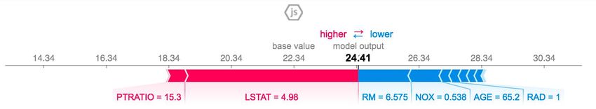
SHAP (SHapley Additive exPlanations)
  One can also interpret single observations:

  The above explanation shows features each contributing to push the model output from the base value to the
 model output (base value: the average model output over the training dataset)
  Features pushing the prediction higher are shown in red, those pushing the prediction lower are in blue

  A stable and reliable implementation of SHAP is available: https://github.com/slundberg/shap

[1] Lundberg and Lee, NIPS 2017, ArXiv: 1705.07874
INTRODUCTION TO DEEP LEARNING // ANGELO ZILETTI, PHD // JANUARY 2021 43

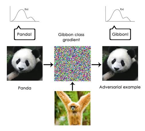
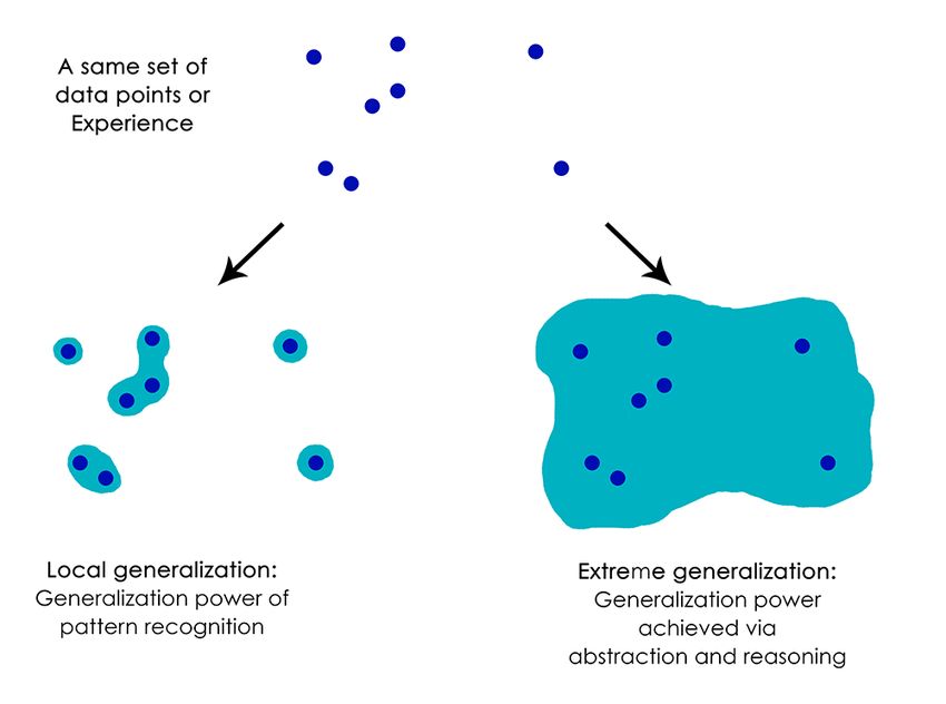
Deep Learning limitations [1]
  “anything that requires reasoning […] is out of reach for deep
 learning models, no matter how much data you throw at them”

  “a deep learning model is just a chain of simple, continuous geometric
 transformations mapping one vector space into another.
  All it can do is map one data manifold X into another manifold Y, assuming
 the existence of a learnable continuous transform from X to Y, and the
 availability of a dense sampling of X:Y to use as training data”

  “One very real risk with contemporary AI is that of misinterpreting what deep
 learning models do, and overestimating their abilities”

 An adversarial example

 [1] F. Chollet, (Keras developer and Google AI researcher): The limitations of deep learning (https://blog.keras.io/the-limitations-of-deep-learning.html)

INTRODUCTION TO DEEP LEARNING // ANGELO ZILETTI, PHD // JANUARY 2021 44

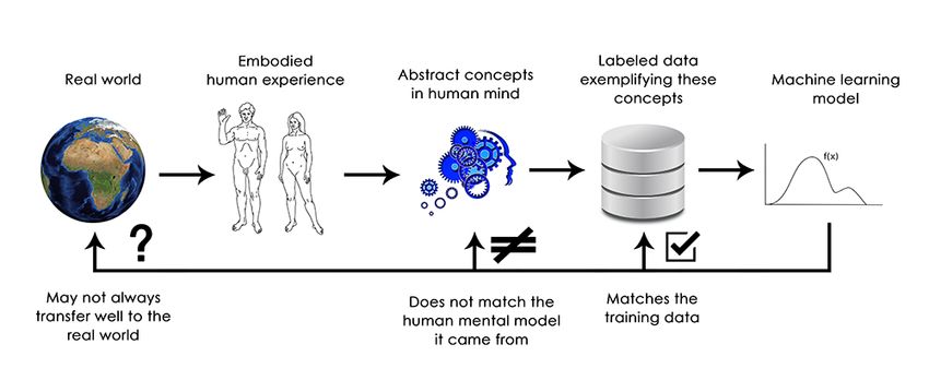
Deep Learning limitations [1]
  “deep learning models do not have any understanding of their input, at least not in any human sense. Our own
 understanding of images, sounds, and language, is grounded in our sensorimotor experience as humans - as embodied
 earthly creatures. Machine learning models have no access to such experiences and thus cannot "understand" their inputs
 in any human-relatable way”

 [1] F. Chollet, (Keras developer and Google AI researcher): The limitations of deep learning (https://blog.keras.io/the-limitations-of-deep-learning.html)

INTRODUCTION TO DEEP LEARNING // ANGELO ZILETTI, PHD // JANUARY 2021 45