A New Reward System Based on Human Demonstrations for Hard Exploration Games
←
→
Page content transcription
If your browser does not render page correctly, please read the page content below
Computers, Materials & Continua                                                                  Tech Science Press
DOI:10.32604/cmc.2022.020036
Article

             A New Reward System Based on Human Demonstrations for
                           Hard Exploration Games
                             Wadhah Zeyad Tareq* and Mehmet Fatih Amasyali

         Faculty of Electrical and Electronics Engineering, Yildiz Technical University, Istanbul, 34220, Turkey
            *
              Corresponding Author: Wadhah Zeyad Tareq. Email: wadhah.zeyad.t.tareq@std.yildiz.edu.tr
                                     Received: 06 May 2021; Accepted: 11 June 2021

                 Abstract: The main idea of reinforcement learning is evaluating the chosen
                 action depending on the current reward. According to this concept, many
                 algorithms achieved proper performance on classic Atari 2600 games. The
                 main challenge is when the reward is sparse or missing. Such environments
                 are complex exploration environments like Montezuma’s Revenge, Pitfall, and
                 Private Eye games. Approaches built to deal with such challenges were very
                 demanding. This work introduced a different reward system that enables the
                 simple classical algorithm to learn fast and achieve high performance in hard
                 exploration environments. Moreover, we added some simple enhancements
                 to several hyperparameters, such as the number of actions and the sam-
                 pling ratio that helped improve performance. We include the extra reward
                 within the human demonstrations. After that, we used Prioritized Double
                 Deep Q-Networks (Prioritized DDQN) to learning from these demonstra-
                 tions. Our approach enabled the Prioritized DDQN with a short learning time
                 to finish the first level of Montezuma’s Revenge game and to perform well
                 in both Pitfall and Private Eye. We used the same games to compare our
                 results with several baselines, such as the Rainbow and Deep Q-learning from
                 demonstrations (DQfD) algorithm. The results showed that the new rewards
                 system enabled Prioritized DDQN to out-perform the baselines in the hard
                 exploration games with short learning time.

                 Keywords: Deep reinforcement learning; human demonstrations; prioritized
                 double deep q-networks; atari

1 Introduction
    Reinforcement learning (RL) achieved many successes in sequential decision-making problems
by adopting the Markov Decision Process (MDP). A famous example of these successes is the
DQN agent [1] that can play Atari games and score higher than the human player in many
of them. Also, RL achieved many successes in hard-exploration domains such as Montezuma’s
Revenge and Pitfall games, in which the rewards are sparse or missing. There are many works
such as DQfD [2], LFSD [3], and Go-explore [4] that used human demonstrations to cover the
problem of spared reward and providing state-of-art in these games.

                      This work is licensed under a Creative Commons Attribution 4.0 International License,
                      which permits unrestricted use, distribution, and reproduction in any medium, provided
                      the original work is properly cited.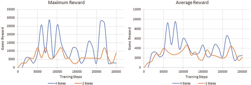
2402                                                                        CMC, 2022, vol.70, no.2

     Many difficulties and limitations on the algorithms that worked to solve hard-exploration
environments made them inappropriate and inapplicable. One of these problems is complexity. All
previous approaches suggested very complex algorithms and techniques that made it challenging
to apply and get the same results. The second problem is the learning time which requires reaching
the required performance. In DQfD, they trained their agent with 200 million steps for each game.
LFSD was needed over two weeks to get the reported result. The last problem is the complexity of
the hardware required to implement these approaches. LFSD used 128 GPU devices to run their
system. Go-explore used sixteen GPUs per run. For these reasons, we wanted to build a simple
system that provides good performance in hard-exploration domains. Furthermore, the system
must be easy to implement and require short learning time with simple devices.
    In this work, we used independent rewards that provide feedback to the agent even when the
environment rewards miss or rare. The environment’s reward was deprecated. These new rewards
are simply covering the problem of sparse and missing rewards. The external rewards implicitly
within the demonstrations. The human demonstrations range from 6,107 to 27,908 transitions.
Our agent learns from a small demonstration compared to other similar work. As DQfD learns
from 10,475 to 35,347 transitions on similar games, AlphaGo [5] learns from 30 million human
transitions. We used Prioritized DDQN, a classical RL algorithm, to learn from these demonstra-
tions. The Prioritized DDQN agent calculates its target network using the Double DQN (DDQN)
algorithm and selecting its experience using a prioritized experience replay (PER) mechanism.
     Also, we showed that the agent’s performance could be enhancement with simple changes in
the game features and algorithms hyper-parameters. For game features, we reduced the number of
the action in the action space. For the hyper-parameters, we increased the ratio of the importance
samples while selecting the examples from the experiences. These two simple enhancements greatly
affected the agent’s performance and improved its results.
    We tested our agent on five different games: Montezuma’s Revenge, Pitfall, Private Eye, Pong,
and Breakout. The performance of our agent in hard-exploration games out-performs pure rein-
forcement learning algorithms DQN, DDQN, Prioritized DDQN, Dueling DDQN, Distributional
DQN, Noisy DQN, and Rainbow. In addition, our agent out-performs the pre-training phase in
DQfD on all five games.

2 Related Work
    Learning from demonstration is essentially concentrated on learning the demonstrator per-
formance. One of the popular algorithms in this field is DAGGER [6]. DAGGER repeatedly
designs new policies depending on polling the demonstrator policy outside its original state space.
That leads to no regret over validation data in the online learning sense. DAGGER asks the
demonstrator to give additional feedback to the agent, which means it requires the demonstrator
to be available during training. In addition, it does not learn to improve beyond the demonstrator.
Deeply AggreVaTeD [7] allows DAGGER to work with continuous robot control and dependency
parsing on raw image data by adding deep neural networks and continuous action spaces. Deeply
AggreVaTeD requires the administrator to be available during the training to provide action and
value function as DAGGER does. Similar to DAGGER, Deeply AggreVaTeD cannot learn to
improve upon the demonstrator.
    Unlike learning from demonstration, reinforcement learning allows the agent to explore in
the environment and learn from trial and error without the need for the demonstrator. Many
RL agents successfully built to learn how to play Atari games. The first deep RL agent was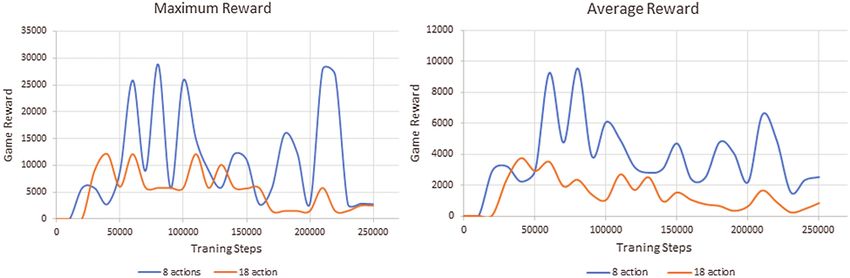
CMC, 2022, vol.70, no.2                                                                           2403

introduced by [8]. The agent learned control policies to play six different games from game frames
and scores only. After that, [1] introduced a notable RL agent, known as DQN, that can play
49 different Atari games and score in many of them higher than the super-human. The DQN saves
the previous experience as a dataset and uses them in training the convolutional neural networks.
This strategy alleviated the correlation and led to superior performance.
     Later works added many improvements to the DQN to enhance the agent’s performance.
Reference [9] proposed adapting the DQN algorithm to reduce the Q algorithm’s overestimation
and increase stable and reliable learning. Their approach is DDQN and used the existing archi-
tecture of the DQN algorithm and the same number of parameters. Reference [10] proposed a
new method for sampling the previous experiences in DQN. Rather than uniformly sampling,
PER proposed to reply to importance transitions more frequently and learn more efficiently.
Reference [11] proposed a new architecture, Dueling Network, for the neural network instead of
the architecture used in all previous works. The dueling network contains two estimators instead
of one estimator in DQN architecture. One of these estimators for the state, and the other is for
the action taken in that state. If the state is not valuable, there is no reason to learn the effect of
each action at each state. A3C [12] presented asynchronous four standard reinforcement learning
algorithms and showed that parallel actor-learners stabilize training, allowing all four methods
to train neural network controllers successfully. Distributional Q-learning [13] learns a categorical
distribution of discounted returns instead of estimating the mean. Noisy DQN [14] uses stochastic
network layers for exploration. Finally, Rainbow [15] combined all six previous extensions of the
DQN algorithm and examined all these extensions’ performance.
    Despite these enhancements, the RL agent is still performing poorly in environments where
the feedback is unavailable or intermittent. Generally, the RL agent learns good policies in many
games where there is feedback from the environment. Many environments do not come with
such features. Montezuma’s Revenge and Pitfall are good examples of such environments. In
these games, the game reward comes after performing a sequence of actions. For covering this
gab, many works suggested using human demonstrations in the learning. Human demonstrations
provide many other advantages like reducing the training time and solve problems that do not
come with accurate simulators.
     DQfD [2] introduced a deep RL agent that uses human demonstrations to learn to play
Atari games. Their algorithm accelerated the learning process and automatically assessed the
necessary ratio of demonstration data. Also, DQfD achieved acceptable results in sparse rewards
environments. Reference [16] train an agent to accomplish the same states seen in a YouTube
video of the game, where [17] combines a sophisticated version of Q-learning to maximize the
likelihood of actions taken in a demonstration. The LFSD [3] also proposed using the human
demonstration to cover the sparse rewards problem in Montezuma’s Revenge games by starting
their agent from demonstration states rather than from the game standard start states. The aim
of this process is to breaks down the complex exploration problem into a curriculum of subtasks.
The Go-explore [4] agent played well in Montezuma’s Revenge and Pitfall games by remembering
the state it visited. The agent is starting the exploration from a new promising state. After that,
it is building the policy by imitation learning.

3 Background
     Learning from demonstrations consists of providing examples of the optimal behavior
(actions). The agent is learning from these demonstrations to behave like the demonstrator even in
new situations. The demonstrating agent is called the expert, and the learning agent is then called
2404 CMC, 2022, vol.70, no.2
the apprentice. This model has already been applied in several fields such as robotics. Generally,
the learning from demonstrations paradigm is placed in the Markov decision process (MDP)
framework. Here the agent solving the problem using a finite set of demonstration instead of
the data generated by itself. The type of guidance used in learning from demonstration is very
different from the one used in RL, which depends mainly on the trial and error [18].
The RL agent must select the correct action among many actions. The main key point in an
RL model that there is no dataset for learning, so there is no answer key. The RL agent must
learn from his own experiences. The only way to evaluate an action is the reward provided by the
environment. The standard MDP becomes a framework for solving RL problems with discrete
actions. The main components of MDP are S, A, R, and S’, where S is a set of states representing
the agent’s current position. A is a set of possible actions that the agent can perform in the
environment. Depending on the selected action, the environment feedbacks the agent with reward
R and transfers the agent from the current state to the next state S’.
The main goal of the agent is to maximize the total reward. For example, in video games, the
total reward accumulates spread rewards from the begging of the game to the final state (game
over). The total reward for one game is
R = r1 + r2 + · · · + rn (1)
The agent must choose the action which returns the highest reward each time. Regarding the
randomness in the environments, a discount factor, γ ∈ [0, 1], is usually used to reduce the reliance
on future rewards [19]. Therefore, the maximum reward is calculating by:
Rt = rt + γ 1 rt+1 + γ 2 rt+2 + · · · + γ n−t rn (2)
To define the maximum future reward as a function of the current state and the action taken
in that state, we can use Q-learning [20]. Now the problem of maximizing the total reward is to
solve the Bellman equation [2]:
∗ ∗
Q (s, a) = E R (s, a) + γ P s | s, a maxa Q s , a (3)
s
where a refers to the next action, Q* is the optimal value function that provides maximal values
in all states. This equation performed using traditional dynamic programming algorithms. In
environments like video games, the state size is large and requires more than one state to represent
the movement directions and speed of the environment objects. DQN [1] solved this problem by
using a deep convolutional neural network. The input is the screen states and outputs the q-value
for each action in the action space. The mean two features that made the DQN agent work are
the separate target network and saving experiences as samples used later in training.
The DDQN update [9] covered the overestimate, which occurs in action values using the
online network to select the action and estimate its value by the target network. The DDQN
target is:
JDQ = R (s, a) + γ Q st+1 , amax
t+1 ; θ (4)
t+1 = argmaxa Q (st+1 , a; θ)
amax (5)
where θ is the weights of the online network, θ
is the weights of the target network. PER [10]
enabled the DQN agent to select the important samples more frequently. These samples are theCMC, 2022, vol.70, no.2 2405
samples that do not fit well with the current estimate of the DQN. These are the samples that
the DQN can learn most from them. Each sample will contain an error. The error is the distance
between the current network output and the target output. The samples and their errors will
store in the agent’s memory, and the errors will update with each learning step. Proportional
prioritization is an approach from PER. In proportional prioritization, the error converted to the
priority depending on this formula:
ps = (error + )α (6)
where epsilon ∈ is a positive number with a minimal value to ensure each sample will assign
to a positive value. The alpha α is a value between 0 and 1. The alpha controls the ratio of
prioritization used. When α equals 0, it means that the samples will select by randomness. The
formula to calculate the probability of being chosen from the error of the sample:
ps
Ps = (7)
k pk
4 Our Agent
The previous RL agents required a long training time until starting to perform an acceptable
behavior. That behavior needs additional learning to be suitable to be used in the real world. This
training time sometimes becomes more expansive than the benefit of the application. In addition
to these disadvantages, the RL agents require complex algorithms and techniques to learn in
environments where the rewards are missed or rare. The goal of our agent is to learn fast using
simple methods to play complex exploration games. Using simple techniques requires feedback
from the environment to enable the agent to evaluate the selected action. To make that possible in
the complex exploration environments, we supplied our agent with an external reward and ignored
the environment feedback.
The external rewards gave to the selected action and the other actions in the action space.
These rewards would give realistic values to all state actions even if the demonstration did not
cover all state space. The realistic values prevent the network from update toward ungrounded
variables. To implement that, in building the demonstrations, we selected only the correct action
and rewarded it with 1, and gave the rest actions in the action space rewards equal to 0.
As we mentioned before, we use simple and already used methods in implementing our
agent. We used the Convolutional neural network CNN from DQN [1]. The CNN contains three
convolutional layers and two fully connected layers with a single output for each action. We
trained the agent with two different sizes of input: four states (St-3, St-2, St-1, St) and two states
(St-1, St). The information with two states enables the agent to perform well but not like the four
states. Also, we trained the agent with a few action numbers for environments that contain many
useless actions. For example, it is enough to play Montezuma’s Revenge game with eight actions
only rather than playing it with eighteen actions. Action’s curtailments helped the agent to learn
faster and perform better.
For calculating the target value, we used the DDQN algorithm. After calculating the target
value, we can find the loss function by applying this equation:
2
JQ = JDQ − Q (s, a; θ) (8)
The second part represents the current output of our model. Finally, we used the proportional
prioritization approach to select the samples from the demonstration data to the mini-batches. In2406 CMC, 2022, vol.70, no.2
previous works, they sampled the important samples with different ratios. In [10], they sampled the
important samples with 60 percent only (α = 0.6). In Rainbow [15], they sampled the important
samples with 50 percent only (α = 0.5). DQfD [2] sampled the important samples with 40 percent
only (α = 0.4). These percent increase annealed linearly to reaching 100 percent, which means
selecting all samples with priority. We selected the important samples with 90 percent (α = 0.9)
and only 10 percent at random for our agent. Also, we increased this percent in the same way.
The reason to select α = 0.9 is that all the samples in the demonstration are important to us, and
we want to learn from all of them. We compared between α = 0.9 and α = 0.6 in one game. Both
the 90 percent and 60 percent allowed our agent to score the same max score but with different
training times. The pseudocode of our agent is showing in Algorithm 1.
Algorithm 1:
1: Input: Dbuffer : empty buffer for storage of the demonstrations. θ: weights for initial behavior
network (random), θ : weights for target network (random), τ : frequency at which to update target
net, st: human demonstrations steps. k: number of training gradient updates.
2: for steps t ∈ {1, 2, . . . st} do
3: Select action by the human player.
4: Play action a on state s and observe (s ).
5: Set the reward of the selected action with r = 1 and the rest with r = 0.
6: Store (s, a, r, s ) into Dbuffer .
7: s ← s
8: end for.
9: for steps t ∈ {1, 2, . . . k} do
10: Sample a mini-batch of n transitions from Dbuffer with prioritization.
11: Calculate loss using the target network.
12: Perform a gradient descent step to update θ.
13: if t mod τ = 0 then θ ← θ end if
14: end for.
5 Our Agent
We now describe the demonstration, hyper-parameters, and setup used for evaluating our
agent.
5.1 Demonstrations
We built our agent to play all Arcade Learning Environment (ALE) [21] games. The ALE
becomes a standard benchmark for RL agents after using it by DQN. Our agent plays the Atari
games from a downsampled 84 × 84 image of the game screen converted to grey-scale as in
previous works. The scores reported are the scores in the Atari game, regardless of how the agent
represents the reward internally.
As we mentioned before, we tested our agent on five different games: Montezuma’s Revenge,
Pitfall, Private Eye, Pong, and Breakout. The human demonstrations are generated by playing the
game and selecting the actions directly from the keyboard. In each step, the environment waits
for us to choose an action that allows us to select the correct actions only without the need for
a super player. We provide demonstrations for each game to our algorithm that we recorded byCMC, 2022, vol.70, no.2 2407
playing the game. For episode number, total steps, and scores obtained in our demonstration for
each game, see Tab. 1.
Table 1: The demonstration episodes number, total steps, and scores for each game
Game Best Worst Transitions Episodes
Montezuma’s revenge 32000 30000 15900 5
Pitfall 35711 3971 27908 5
Private eye 20700 20300 8636 5
Breakout 79 17 10289 9
Pong 1 −1 6107 3
5.2 Evaluation Methodology
The previous works evaluated their agents in two ways. The first way is evaluating the
agent during training to find the best agent snapshot, such as in [1,9], and [15], where they are
suspending the learning after every one million steps and evaluated the last weights for 500K
steps. The second way [15] is by taking the best agent snapshot and re-evaluated it by testing it
on many episodes and taking the average game score in all episodes.
In this paper, we trained our agent for 250K steps only. We saved and updated the weights
after each 10K steps. At the end of the training, we have 25 different weights. To find the best
agent snapshot (best weight), we test each weight for each game on ten episodes, and we took the
maximum and average score for these ten episodes. Result section showing the maximum and the
average score per weight for each game.
5.3 Comparison to Published Baselines
We compared our results to the popular baseline published algorithms: DQN, DDQN, Prior-
itized DDQN, Dueling DDQN, Distributional DQN, Noisy DQN, and Rainbow. It is impossible
to train and test all these algorithms on our devices due to the hardware features and training
time requirements. To achieve a fair comparison, we followed the same evaluation settings of
the published results that we took from [15]. Also, we compared our agent with the phase one
agent from the DQfD algorithm on the same games with the same demonstrations. Many reasons
enabled us to train and test the agent from DQfD phase one:
• The agent is learning from human demonstrations only in phase one.
• The training time is 750,000, which is a short time compared with other baselines requiring
about 200 million steps.
• The memory size requires during the training is small. During phase one, only the demon-
strations need to store. On the other baselines, they kept 1 million samples which impossible
to implement with our device.
5.4 Hyper-Parameters
Here are the parameters used for our algorithm. For the DQfD agent, we followed the
parameters in the original paper.
• Pre-training steps k = 250,000 mini-batch updates.2408 CMC, 2022, vol.70, no.2
• Batch size n = 32.
• γ = 0.99.
• Prioritized replay importance sampling exponent α = 0.9.
• Prioritized replay constants = 0.01.
• Target network update period τ = 10,000.
• RMSprop learning rate = 0.00025.
• Target network update frequency = 10000.
Finally, the machine which we used to train algorithms is simple. It contains 6 CPU cores,
16 GB of RAM with a single GPU device. The GPU device is Nvidia GTX 1060 (6 GB memory).
6 Result and Discussion
First, we compared the performance of the agent with and without the enhancements that we
added. For enhancements comparison, we used Montezuma’s Revenge game only. We have three
different comparisons: eighteen vs. eight actions number, 0.6 PER vs. 0.9 PER, and four states
vs. two states input size. Fig. 1 showing the results of testing the agent with eight actions and
eighteen actions. The maximum score for the eighteen actions is 12,100, and the agent could not
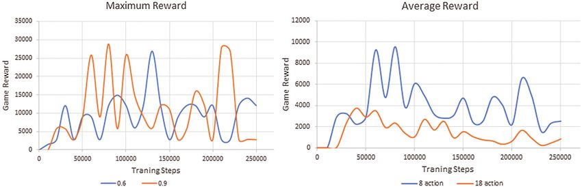
finish the first level compared with the eight action results. Fig. 2 shows the results of testing the
agent by selecting important samples with 0.9 and 0.6 rates. The agent with 90 percent scored the
maximum reward after only 50,000 updates, while it requires 120,000 updates to achieve it with
60 percent. Finally, Fig. 3 shows the difference between using four states and two states as an
input to CNN. It is common to use four frames to represent the state of the games in all RL
works. The four states can determine the direction and the speed of the objects on the screen. It
is successful to use only two frames to represent the state of the game. The agent can play the
game, scoring very acceptable results but with a maximum score of 12,100.
Figure 1: Different between 8 actions and 18 action results. The left plot shows the maximum
scores. The right plot shows the average scores
Figs. 4–8 shows the maximum and average reward for our agent on Montezuma’s Revenge,
Pitfall, Private Eye, Breakout, and Pong games with eight actions, 0.9 PER, and four input states.
The Pong contains six actions, and the Breakout game has four actions only. So, it is unnecessary
to reduce their action number.CMC, 2022, vol.70, no.2 2409
Figure 2: Different between 0.9 PER and 0.6 PER results. The left plot shows the maximum
scores. The right plot shows the average scores
Figure 3: Different between input with four states and two states results. The left plot shows the
maximum scores. The right plot shows the average scores
In Montezuma’s Revenge game, our agent required only 80,000 steps of training to its
maximum score of 28,900. This score is meaning that the agent successfully finished the first
level of the game. The weight with 80,000 training steps is the best snapshot of the agent in
Montezuma’s Revenge game. In the Pitfall game, our agent has a more stable performance. The
agent required only 60,000 steps of training time to its maximum score of 7782. The weight with
60,000 training steps is the best snapshot of the agent in the Pitfall game. In the Private Eye game,
the performance of the agent is excellent. The agent required only 40,000 steps of training time
to scoring even higher than the demonstration score. In demonstrations of the game, the higher
score was 20,700. The higher score of the agent is 28,374. Also, each weight of the 25 weights
can score the maximum score of the demonstrations. The weight with 40,000 training steps is the
best snapshot of the agent in the Private Eye game.2410 CMC, 2022, vol.70, no.2 Figure 4: Maximum and average scores for our agent on Montezuma’s revenge game. The gray area represents the minimum and maximum scores of the demonstrations used in training Figure 5: Maximum and average scores for our agent on the Pitfall game. The gray area represents the minimum and maximum scores of the demonstrations used in training
CMC, 2022, vol.70, no.2                                                              2411

Figure 6: Maximum and average scores for our agent on the private eye game. The gray area
represents the minimum and maximum scores of the demonstrations used in training

Figure 7: Maximum and average scores for our agent on the breakout game. The gray area
represents the minimum and maximum scores of the demonstrations used in training
2412                                                                       CMC, 2022, vol.70, no.2

Figure 8: Maximum and average scores for our agent on the pong game. The gray area represents
the minimum and maximum scores of the demonstrations used in training

     The performance of our agent is not good in environments where the reward available. We
trained and tested our agent on two popular games, Breakout and Pong. The classical RL algo-
rithms achieved perfect performance in these environments. Unlike the hard-exploration games, the
states of these two simple environments changing depending on each action, and it is impossible to
cover all these states with the demonstrations. However, our agent’s performance is good compared
to the duration of training and demonstration size. For the Breakout game, our agent scored 31
as a maximum score with 240,000 steps of training. The weight with 240,000 training steps is
the best snapshot of the agent in the Breakout game. For the Pong game, our agent scored −10
(our agent scored 11 from 21 total scores) after 20,000 steps of training. The weight with 20,000
training steps is the best snapshot of the agent in the Pong game.
    As we mentioned before, we compared our results to the popular baseline published algo-
rithms: DQN, DDQN, Prioritized DDQN, Dueling DDQN, Distributional DQN, Noisy DQN,
and Rainbow. Also, we compared our agent with the DQfD agent (phase 1) that we trained in
our device with the same training period in the original paper (750,000 steps). To achieve a fair
comparison, we followed the same evaluating procedure of the published results that we took
from [15]. We test our best agent snapshot that we obtained previously and the DQfD agent that
we trained on 200 episodes, and we started each episode with up to 30 no-op actions. For results,
see Tab. 2.
     Our agent out-performs all the other baselines in all hard explore environments that we
selected. Of course, the average results of the 200 episodes were lower than the average of the
ten episodes shown in previous Figs. 4–8. Due to the 30 no-op actions and the number of the
episodes. The DQfD agent out-performs the baseline performance in the Private Eye game only.
The score of the DQfD agent published in their manuscript is much higher than the results shown
in Tab. 2. The reason is that we trained the DQfD agent for 750,000 steps only for each game
while they reported their results after 200 million steps of training.
CMC, 2022, vol.70, no.2 2413
Table 2: No-op starts evaluation regime: Raw scores across all games averaged over 200 testing
episodes from the agent snapshot that obtained the highest score during training. We report
the published scores for DQN, DDQN, prioritized DDQN, dueling DDQN, distributional DQN,
Noisy DQN, and rainbow. For DQfD and our agents, we report our evaluations of the agents
Game Montezuma’s revenge Pitfall Private eye Pong Breakout
DQN 0.0 −286 146 19.5 385.5
DDQN 0.0 −29.9 129 20.9 418.5
PDDQN 0.0 0.0 200 20.7 381.5
Duel DDQN 0.0 0.0 103 21.0 345.3
Distrib DQN 384 −2.1 15172 20.8 612.5
Noisy DQN 206 −18.2 3966 21.0 459.1
Rainbow 384 0.0 4234 20.9 417.5
DQfD 206 265 8438 −19.5 1.99
Our agent 5035 2034.3 23152 −14.5 2.39
Our agent performance is not good in simple environments comparing with the baselines.
However, it is still providing better performance than the DQfD agent. DQfD agent has needed
200 million steps of training to achieve good performance in such games.
7 Conclusion
The traditional RL algorithms faced a grand challenge in hard-exploration environments.
The alternative algorithms were complex and hard to implement. This work proposes a new
approach that enables the Prioritized DDQN, a traditional RL algorithm, to perform well in such
environments. The main idea of our approach is to cover the problem of missing rewards by
implying external rewards in human demonstrations and using those demonstrations to train the
RL algorithm. The result showed the ability of the Prioritized DDQN algorithm with the external
rewards to play different hard-exploration environments. Furthermore, the new approach reduces
training time and requires simple machines to be implemented compared with previously published
approaches.
Funding Statement: The authors received no specific funding for this study.
Conflicts of Interest: The authors declare that they have no conflicts of interest to report regarding
the present study.
References
[1] V. Mnih, K. Kavukcuoglu, D. Silver, A. A. Rusu, J. Veness et al., “Human-level control through deep
reinforcement learning,” Nature, vol. 518, no. 7540, pp. 529–533, 2015.
[2] T. Hester, M. Vecerik, O. Pietquin, M. Lanctot, T. Schaul et al., “Deep q-learning from demonstra-
tions,” in Proc. of the 32nd AAAI Conf. on Artificial Intelligence, Louisiana, USA, vol. 32, pp. 3223–3230,
2018.
[3] T. Salimans and R. Chen, “Learning montezuma’s revenge from a single demonstration,” in Proc. of
the 32nd Conf. on Neural Information Processing Systems NIPS, Montréal, Canada, 2018.
[4] A. Ecoffet, J. Huizinga, J. Lehman, K. O. Stanley and J. Clune, “Go-explore: A new approach for
hard-exploration problems,” arXiv preprint arXiv, vol. 1901.10995, pp. 1–37, 2019.2414 CMC, 2022, vol.70, no.2
[5] D. Silver, A. Huang, C. J. Maddison, A. Guez, L. Sifre et al., “Mastering the game of go with deep
neural networks and tree search,” Nature, vol. 529, no. 7587, pp. 484–489, 2016.
[6] S. Ross, G. J. Gordon and J. A. Bagnell, “A reduction of imitation learning and structured prediction
to no-regret online learning,” in Proc. of the 14th Int. Conf. on Artificial Intelligence and Statistics, Fort
Lauderdale, FL, USA, vol. 15, 2011.
[7] W. Sun, A. Venkatraman, G. J. Gordon, B. Boots and J. A. Bagnell, “Deeply aggrevated: Differentiable
imitation learning for sequential prediction,” in Proc. of the Int. Conf. on Machine Learning, Sydney,
Australia, pp. 3309–3318, 2017.
[8] V. Mnih, K. Kavukcuoglu, D. Silver, A. Graves, I. Antonoglou et al., “Playing atari with deep
reinforcement learning,” arXiv preprint arXiv, vol. 1312.5602, pp. 1–9, 2013.
[9] H. V. Hasselt, A. Guez and D. Silver, “Deep reinforcement learning with double q-learning,” in Proc.
of the 30th AAAI Conf. on Artificial Intelligence, Arizona, USA, vol. 30, pp. 2094–2100, 2016.
[10] T. Schaul, J. Quan, I. Antonoglou and D. Silver, “Prioritized experience replay,” in Proc. of the Int.
Conf. on Learning Representations, San Juan, Puerto Rico, 2016.
[11] Z. Wang, T. Schaul, M. Hessel, H. V. Hasselt, M. Lanctot et al., “Dueling network architectures for
deep reinforcement learning,” in Proc. of the 33rd Int. Conf. on Machine Learning, New York, NY, USA,
vol. 48, 2016.
[12] V. Mnih, A. P. Badia, M. Mirza, A. Graves, T. Harley et al., “Asynchronous methods for deep
reinforcement learning,” in Proc. of the 33rd Int. Conf. on Machine Learning, New York, NY, USA,
vol. 48, 2016.
[13] M. G. Bellemare, W. Dabney and R. Munos, “A distributional perspective on reinforcement learning,”
in Proc. of the 34th Int. Conf. on Machine Learning, Sydney, Australia, vol. 70, 2017.
[14] M. Fortunato, M. G. Azar, B. Piot, J. Menick, M. Hessel et al., “Noisy networks for exploration,” in
Proc. of the Int. Conf. on Learning Representations, British Columbia, Canada, 2018.
[15] M. Hessel, J. Modayil, H. V. Hasselt, T. Schaul, G. Ostrovski et al., “Rainbow : Combining improve-
ments in deep reinforcement learning,” in Proc. of the 32nd AAAI Conf. on Artificial Intelligence,
Louisiana, USA, vol. 32, pp. 3215–3222, 2018.
[16] Y. Aytar, T. Pfaff, D. Budden, T. L. Paine, Z. Wang et al., “Playing hard exploration games by watching
YouTube,” in Proc. of the 32nd Conf. on Neural Information Processing Systems, Montréal, Canada, 2018.
[17] T. Pohlen, B. Piot, T. Hester, M. G. Azar, D. Horgan et al., “Observe and look further: Achieving
consistent performance on atari,” arXiv preprint arXiv, vol. 1805.11593, pp. 1–19, 2018.
[18] B. Piot, M. Geist and O. Pietquin, “Bridging the gap between imitation learning and inverse rein-
forcement learning,” IEEE Transactions on Neural Networks and Learning Systems, vol. 28, no. 8,
pp. 1814–1826, 2017.
[19] J. Wang, L. Gou, H. Shen and H. Yang, “DQNViz: A visual analytics approach to understand deep
q-networks,” IEEE Transactions on Visualization and Computer Graphics, vol. 25, no. 1, pp. 288–298,
2019.
[20] C. J. C. H. Watkins and P. Dayan, “Q-learning,” Machine Learning, vol. 8, no. 3–4, pp. 279–292, 1992.
[21] M. G. Bellemare, Y. Naddaf and J. Veness, “The arcade learning environment: An evaluation platform
for general agents,” Journal of Artificial Intelligence Research, vol. 47, pp. 253–279, 2013.You can also read