Processing Satellite Imagery for Decision-Making in Precision Agriculture
←
→
Page content transcription
If your browser does not render page correctly, please read the page content below
Processing Satellite Imagery for Decision-Making in
                            Precision Agriculture
                            Panagiotis Bouros                                                                     Ira Assent
                  Institute of Computer Science                                                   Department of Computer Science
         Johannes Gutenberg University Mainz, Germany                                               Aarhus University, Denmark
                      bouros@uni-mainz.de                                                                  ira@cs.au.dk

                      Jacob Høxbroe Jeppesen                                                   Thomas Skjødeberg Toftegaard
                       Department of Engineering                                                     Department of Engineering
                       Aarhus University, Denmark                                                    Aarhus University, Denmark
                             jhj@eng.au.dk                                                                 tst@eng.au.dk

ABSTRACT                                                                            context is captured by object geometries and their distance in
Empowered by geo-locating and sensor-based technologies, pre-                       space. Finally, a collective outlier is a group of clustered objects
cision agriculture brings a data-intensive paradigm into farming.                   with low variance among them, which are together inconsistent
In this spirit, we investigate the role of outlier detection and                    to the rest of the dataset.
visualization in decision-making for precision agriculture. We                          In precision agriculture, outlier detection is mainly studied for
discuss two analysis tasks for visually monitoring fields that ex-                  pre-processing and cleaning of the collected data [13]. The focus
hibit problematic crop growth compared to their neighbors, and                      has been on detecting errors introduced by measurement failures,
for visualizing problematic areas inside a field. As a proof of                     e.g., related to the accuracy and the calibration of sensor and po-
concept, we analyze satellite imagery to case-study our tasks in                    sitioning devices, or even to signal loss. In contrast, anomalies
the context of the Future Cropping project.                                         directly related to poor decision-making, e.g., crop establishment,
                                                                                    fertilization or herbicide application, and to natural causes in-
                                                                                    cluding climate, topography, and soil-landscape features, have
1    INTRODUCTION                                                                   received less attention.
The proliferation of the Global Positioning System (GPS) and of                         In an attempt to fill this gap, we propose the tasks of inter-field
sensor-based technologies have given rise to a different paradigm                   (i.e., between fields) and intra-field (i.e., within a field) analy-
of agriculture. Precision agriculture as this paradigm is known,                    sis. In the former, our goal is to identify fields, which exhibit a
strikes to improve economic returns and reduce the environmen-                      problematic behavior, e.g., unexpectedly low collected crop mass,
tal impact [4, 7–9]. Harvesters mounted with sensors and GPS                        compared to their neighboring fields. 1 The key challenges for
receivers allow for instant collection of position-aware crop data.                 this task are twofold; (i) how to define field neighborhood and (ii)
Contemporary Geographic Information Systems (GIS) are able to                       how to quantify the importance/influence of each neighbor. Dif-
store and analyze collected crop data, in many cases combined                       ferent from traditional spatial outlier detection that relies solely
with other types of information from multiple sources such as                       on arbitrary polygon distances, we consider domain-specific data
satellites and meteorological stations. Decision-making plays a                     properties such as soil/crop type and the variation of crop-growth.
key role in the effort of exploiting this abundance of data. Tradi-                 On the other hand, intra-field analysis is triggered in an effort to
tionally, decision-making heavily relies on farmers’ experience                     interpret the results of inter-field analysis. The goal is to identify
and empirical knowledge. In contrast, in precision agriculture,                     and visualize the areas inside a particular problematic field that
information is quantified and decision-making is supported by a                     significantly deviate from the average or normal behavior of the
systematic and data-intensive analytical procedure that can be                      field. Practically, these are the areas where the farmer may need
visualized for novel insights and improved farming decisions.                       to take action [4, 7], e.g., by increasing fertilization, changing
   Anomaly or outlier detection has been widely studied in data                     crop type or building drains. Overall, the proposed tasks are
mining to support decision-making; the goal is to identify objects                  of great value not only to farmers but also to contractors and
that significantly deviate from the expected pattern in a dataset                   consultants of agriculture.
[1]. There exist essentially three types of ourliers. Point outliers                    Recent studies [5, 6] showed how precision agriculture may
generally studied in multidimensional data management, are ob-                      benefit from processing satallite imagery. Imagery datasets have
jects inconsistent with the rest of the dataset. Detection of this                  become readily available by open access to NASA Landsat in
type mainly involves statistical and distribution-based methods.                    2008 [14] and to ESA Sentinel satellites. In line with this trend,
Contextual outliers are defined based on a set of contextual and                    we conduct a case study for our inter- and intra-fields tasks in
behavioral attributes; these objects exhibit significantly different                the context of the Future Cropping project. Our study employs
values on their behavioral attributes compared to dataset objects                   satellite imagery in two manners. First, we calculate a vegetation
with similar values on the contextual attributes. The key for con-                  index to monitor the crop growth on the fields. Second, our intra-
textual outlier detection is to identify those objects with similar                 field task properly partitions a field to take full advantage of the
contextual attributes also known as the neighborhood of an object.                  detail and the resolution of the available imagery data.
Spatial outliers [12] are a type of contextual outliers where the

© 2019 Copyright held by the author(s). Published in the Workshop Proceedings of
the EDBT/ICDT 2019 Joint Conference (March 26, 2019) on CEUR-WS.org. Distri-        1 Note
bution of this paper is permitted under the terms of the Creative Commons license         that besides problematic, we can also identify fields that outperform their
CC-by-nc-nd 4.0.                                                                    neighbors; in other words, we are able to detect both negative and positive outliers.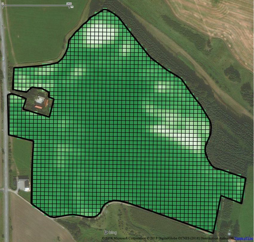
Table 1: Notation                                       then field f behaves worse than expected based on its neighbor-
                                                                                      hood; we call f a negative outlier in this case. Otherwise, f is
       symbol          description                                                    a positive outlier that exceeds our expectations. Both cases are
      α                Attribute of interest                                          important for decision-making in precision agriculture as nega-
    f .α               Value for the attribute of interest on field f                 tive outliers may require immediate action by the farmers and
    f . αb             Predicted value for the attribute of interest on field f       positive outliers may provide important feedback to improve
     Nf                Neighborhood of field f                                        crop growth in other fields.
     wi                Weight of neighbor field n i
     Pf                Partitioning of field f
    p .α               Value for the attribute of interest on partition p
                                                                                      2.2      Intra-field Analysis
 dist (f 1, f 2 )      Spatial distance between fields f 1 and f 2                    Conceptually, the process of intra-field analysis involves three
 M AX _DI ST           Maximum allowed distance between two fields                    steps. First, the extent of each field is split into a number of
                                                                                      partitions; each partition represents an area of interest. In practice,
                                                                                      such a partitioning may for instance be provided by the farmer
2       ANALYSIS TASKS                                                                or generated by a partitioning process. For instance, in our case
Besides spatial geometries (e.g., polygons and/or point data), our                    study of Section 3, we used the image resolution to partition our
outlier detection methodology uses for every field (or parts of                       satellite data. Similar to the entire field, we assume that each
it) a set of numerical attributes that store measurements such as                     partition is associated with the same attribute of interest α. 3
the collected crop mass, and a set of categorical attributes which                    We next define |pi .α − f .α | as the deviation of α’s value on a
store properties of the field such as its soil and crop type. Our                     particular partition pi , from the value on the entire field f . Last,
analysis focuses on a particular numerical attribute of interest                      we can employ the two approaches discussed in the previous
denoted by α, which monitors the crop growth on a field; Table 1                      subsection for the inter-field analysis to report the outlying areas
summarizes the notation used throughout the rest of this paper.                       of a field, i.e., either by ranking the partitions by their |pi .α − f .α |
                                                                                      deviation value, or by reporting the partitions with an extreme
                                                                                      deviation value.
2.1        Inter-field Analysis
We model inter-field analysis as a spatial outlier detection task                     3     CASE-STUDY
[12] with attribute of interest α as the behavioral attribute of
                                                                                      We case-studied our outlier detection tasks for the inter- and the
our analysis while the geometry (polygon), the categorical at-
                                                                                      intra-field analysis in the context of the Future Cropping project,
tributes and the rest of the numerical attributes are the contextual
                                                                                      which collects and analyzes agricultural data in Denmark. 4 Our
attributes used to define the neighborhood around each field.
                                                                                      study involves two types of data; (i) the geometries (i.e., the
   Conceptually, the process of inter-field analysis involves three
                                                                                      polygons) of all 590,490 fields in Denmark and their crop type,
steps. First, the neighborhood of each field f is defined on the
                                                                                      and (ii) a 6.3GB vegetation map derived from ESA Sentinel-2
basis of the contextual attributes. Under this, selecting the proper
                                                                                      satellite imagery captured on May 8, 2016. 5 We conducted our
distance measure dist between two fields is critical; dist takes
                                                                                      case-study on QGIS. 6
into account the spatial proximity of the fields and potentially
the values of other contextual attributes, e.g., the soil type. Let
                                                                                      3.1      Processing Satellite Imagery
N f be the set of neighbors for a field f . The second step is to
predict the value for the attribute of interest α on f by aggregat-                   In the past, a number of vegetation indices [2, 3, 10, 11] has been
ing the values on f ’s neighbor fields in N f ; typically, the mean                   proposed to monitor the crop growth on fields, primarily by
value is used for this purpose. 2 In our study, we calculate f .b
                                                                α as                  estimating properties of vegetation such as the concentration
the weighted mean value, which allows us to weight the impor-                         of biomass or chlorophyll. Similar to previous studies [5, 6], we
tance and the contribution of each neighbor, considering both                         consider the Normalized Difference Vegetation Index (N DV I ) for
the spatial distance to field f and other factors as discussed in                     our case-study. ESA Sentinel-2 satellites provide 13-band multi-
Section 3.2. Formally, we have:                                                       spectral images with a spatial resolution down to 10m × 10m.
                                                                                      N DV I values can be calculated combining two particular spectral
                                      |N |                                            bands:
                                    Σi=1f {w i · ni .α }
                            f .b
                               α=                                              (1)                                      N IR − V IR
                                             |N |                                                            N DV I =                                  (2)
                                         Σi=1f w i                                                                      N IR + V IR
                                                                                      where N IR and V IR are the near-infrared and the visible red
where w i denotes the weight of neighbor field ni . The third step                    bands, respectively.
is to report the outlying fields. The value of | f .bα − f .α | quantifies               For our analysis, we use N DV I as the attribute of interest α.
the deviation of α’s predicted value from the actual value on a                       Specifically, we first calculate the index value on every pixel of
field f . In practice, there exist two approaches for determining                     the satellite images using Formula 2. Then, for each field f , we
outliers. We can either rank the fields in decreasing order of their                  compute mean µ f and standard devation σf of its N DV I values
| f .b
     α − f .α | deviation and output the top k, or return all fields with             based on the overlapping pixels, and set f .α = µ f . Figure 1b
an extreme deviation value. Probabilistic and statistical models
can be used to determine such extreme deviation values [1].                           3 Essentially, the value of attribute α on both the entire field and a partition is
     The above procedure allows us to identify fields whose pre-                      computed by aggregation. For instance, harvesters store position-aware crop data for
                                                                                      the collected mass on specific geographic locations inside a field; we can aggregate
dicted value on attribute of interest α significantly deviates from                   these values to compute the overall collected mass for the entire field or for particular
the actual value. In fact, we distinguish between two types of out-                   areas.
                                                                                      4 https://futurecropping.dk
liers based on the sign of the f .bα − f .α deviation. If f .b
                                                             α − f .α > 0             5 https://kortdata.fvm.dk/download/Index?page=Markblokke_Marker,
                                                                                      https://scihub.copernicus.eu
2 As   an alternative, median can be used to smooth the impact of extreme α values.   6 https://qgis.org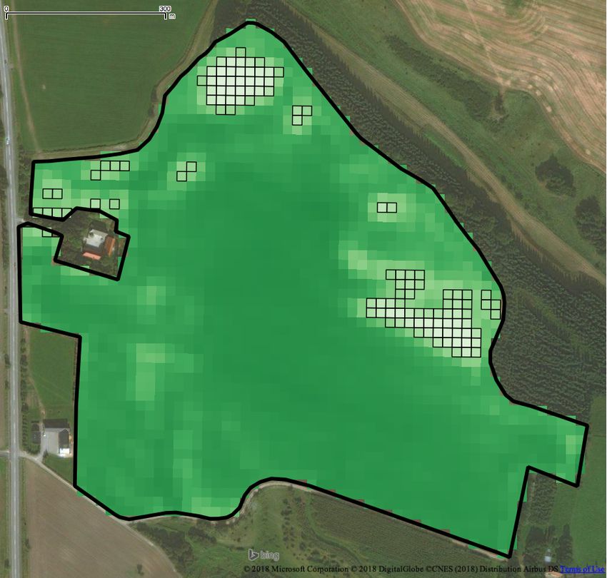
(a) (b)
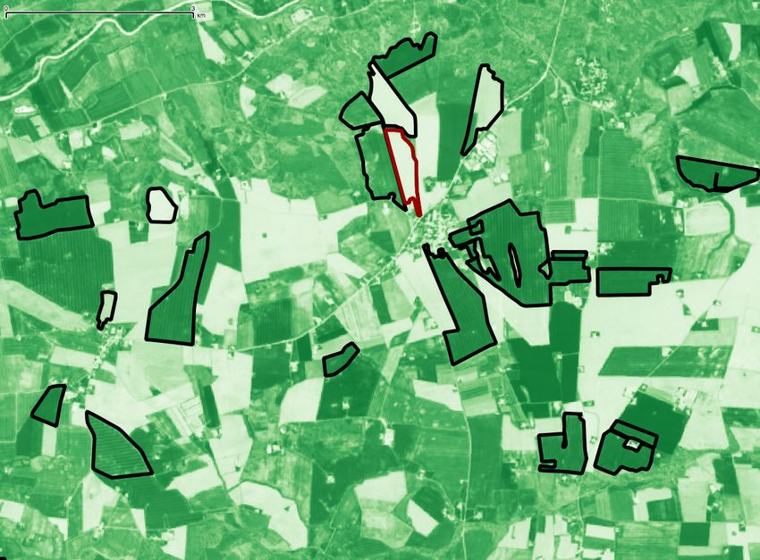
Figure 1: Inter-field analysis on winter rapeseed crop fields: (a) distribution of f .b
α − f .α values with mean value µd = 0.0013
and standard deviation σd = 0.1645, (b) example of a negative outlier (in red) with f .α = 0.176 and f .b α = 0.671.
Table 2: Top-10 most important neighbors of f in Fig- grown on their entire extent. These are fields with a similar N DV I
ure 1b. value (visually, with a similar shade of green) on the majority of
their overlapping pixels; hence, low variance in crop growth for
field α (N DV I ) dist(f , ni ) (in meters) σi wi
neighbor ni can be captured by a low σi standard deviation of
f 0.176 – – – the N DV I values. Formally, weight w i is defined as:
n1 0.183 14 0.071 0.928
dist(f , ni )
n2 0.764 264 0.054 0.921 wi = 1 − · [1 − σi ] (4)
n3 0.762 311 0.056 0.914 MAX _DIST
n4 0.777 452 0.056 0.901 With Formulas 1, 3 and 4, we compute the f .b α − f .α deviation
n5 0.724 435 0.059 0.900 of the predicted value from the actual f .α N DV I value, on every
n6 0.604 75 0.098 0.895 field f . As discussed in Section 2.1, one option for our inter-field
n7 0.629 5 0.110 0.889 analysis, would be to rank all fields by their deviation and rec-
n8 0.753 1,277 0.067 0.814 ommend the ones with the k highest values as potential negative
n9 0.787 1,644 0.028 0.813 outliers and those with the k lowest deviation values as positive
n 10 0.347 408 0.169 0.797 outliers. However, such recommendations have little practical
merit for the end-user; for instance, even the highest f .b α − f .α
value may in fact be too low to mark field f as problematic. In-
shows a snapshot of our N DV I map for the fields in Denmark;
stead, we focus on identifying the fields that exhibit the most
the greener a field (or parts of it) appears, the higher its f .α (i.e.,
extreme deviation values.
N DV I ) value is.
Figure 1a reports on the distribution of the f .b α − f .α values for
a particular type of crop called winter rapeseed. The mean value
3.2 Inter-field Analysis and the standard deviation for this distribution are µd = 0.0013
We now present our case-study for the inter-field analysis and and σd = 0.1645, respectively. We observe that over 99.5% of
exemplify its results. We apply Formula 1 on each field f in the fields have a f .b α − f .α value inside [µd −3·σd , µd +3·σd ]. A
Denmark to predict its N DV I value, i.e., f .b α . For performance, similar conclusion was drawn for the rest of the crop types in
previous works in outlier detection typically define neighbor- our case-study. Based on this observation, we follow a typical
hood N f as the k closest fields. However, these neighbors (or statistical approach for identifying extreme f .b α − f .α values [12],
part of them) could be in fact very distant to field f , which will namely those that deviate from mean µd at least three times the
potentially affect the quality of the results. Instead, we narrow |f . αb−f .α −µ d |
standard deviation σd , i.e., σd ≥ 3 holds. 8 The nature
the extent of a neighborhood; hence, N f contains all fields of the
of the outlier (positive or negative) is determined by the sign of
same crop type as f within a radius of 10km, as suggested by our
f .b
α − f .α.
agricultural project partners. Formally, we define the distance of
Figure 1b visually exemplifies our inter-field analysis for the
f to a neighbor field ni as:
( winter rapeseed crop; the negative outlier field f is highlighted by
ED(f , ni ) if fields f , ni have same crop type a red border while a subset of its neighborhood is given in black.
dist(f , ni ) =
MAX _DIST otherwise Further, Table 2 lists the characteristics of the 10 most important
(3) neighbors of f , sorted by their weight w i (Formula 4); notice how
where ED(f , ni ) is the Euclidean distance of fields f , ni polygons the closest field to f , n 7 , is not its most important neighbor as
and MAX _DIST is the maximum 10km distance. n 7 exhibits a higher variation of crop growth compared to fields
To weight the importance of a neighbor ni ∈ N f , we take into n 1 to n 6 . For field f , we have its actual N DV I value f .α = 0.176
account two factors; (1) its spatial distance dist(f , ni ) to f and while using Formula 1, we predict that f .b α = 0.671. The extreme
(2) the variation of crop growth inside the field. 7 Essentially, we deviation of the predicted from the actual N DV I value is captured
prioritize neighbors located close to field f , with crops evenly in Figure 1b where the majority of the shown neighbors are
7 The 8 Note that µ d , σd are statistics computed for the particular crop type of field f .
importance of low-variation fields has been previously studied e.g., in [5].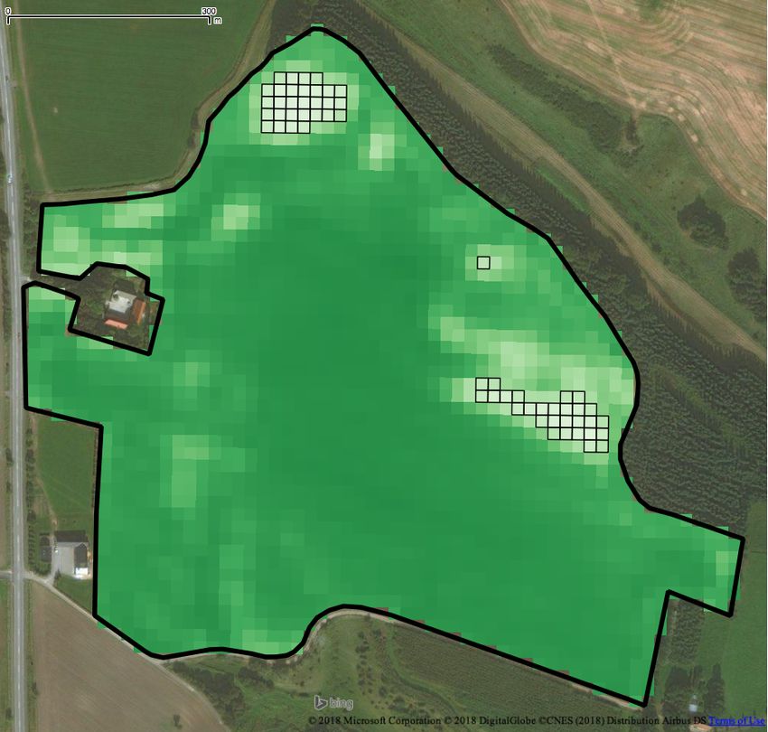
deviation σd . Observe how our analysis is able to report the
                                                                          partitions that cover the light colored problematic areas of the
                                                                          field. Additional problematic areas can be identified by reporting
                                                                          partitions with a |pi .α − f .α | value deviating 2 times, as shown
                                                                          in Figure 2c.

                                                                          4     CONCLUSIONS
                                                                          We studied the role of outlier detection in decision-making for
                                                                          precision agriculture and how such tasks can benefit from pro-
                                                                          cessing satellite imagery. For this purpose, we discussed the tasks
                                                                          of inter- and intra-field analysis, addressing the special challenges
                                                                          raised by the agricultural domain. As a proof of concept, we con-
                                                                          ducted a case-study supported by ESA satellite images within
                                                                          the Future Cropping project.
                                                                              In the future, we plan to extend our study in multiple direc-
                                                                          tions; (i) incorporate more types of data, e.g., collected from har-
                                                                          vesters or rain distribution data, (ii) employ visualization tools to
                                                                          collect and evaluate farmers’ feedback, (iii) enhance intra-field
                                                                          analysis for recommending explicit actions to farmers, (iv) fur-
                                                                          ther analyze satellite imagery to monitor the outlying fields or
                                                                          problematic areas through the course of time and (v) investigate
                                                                          techniques from Machine Learning for predictive analytics.

                                                                          ACKNOWLEDGEMENTS
                                                                          This work was funded by Innovation Fund Denmark as part of
                                                                          the Future Cropping project (J. nr. 5107-00002B).

                                                                          REFERENCES
                                                                           [1] Charu C. Aggarwal. 2013. Outlier Analysis. Springer. https://doi.org/10.1007/
                                                                               978-1-4614-6396-2
                                                                           [2] Jan G.P.W. Clevers, Steven M. de Jong, Gerrit F. Epema, Freek van der Meer,
                                                                               Wim H. Bakker, Andrew K. Skidmore, and Elisabeth A. Addink. 2001. MERIS
                                                                               and the red-edge position. International Journal of Applied Earth Observation
                                                                               and Geoinformation 3, 4 (2001), 313 – 320.
                                                                           [3] Anatoly A. Gitelson, Yoram J. Kaufman, and Mark N. Merzlyak. 1996. Use
                                                                               of a green channel in remote sensing of global vegetation from EOS-MODIS.
                                                                               Remote Sensing of Environment 58, 3 (1996), 289 – 298.
                                                                           [4] Peter. Skøjdt, Poul Møller Hansen, and Rasmus Nyholm Jørgensen. 2003. Sensor
                                                                               Based Nitrogen Fertilization Increasing Grain Protein Yield in Winter Wheat.
                                                                               Technical Report Risø-R-1389. Risø National Laboratory, Roskilde, Denmark.
                                                                           [5] Jacob Høxbroe Jeppesen, Rune Hylsberg Jacobsen, Rasmus Nyholm Jørgensen,
                                                                               Andes Halberg, and Thomas Skjødeberg Toftegaard. 2017. Identification
                                                                               of High-Variation Fields based on Open Satellite Imagery. 11th European
                                                                               Conference on Precision Agriculture.
                                                                           [6] Jacob Høxbroe Jeppesen, Rune Hylsberg Jacobsen, Rasmus Nyholm Jørgensen,
                                                                               and Thomas Skjødeberg Toftegaard. 2016. Towards Data-Driven Precision
Figure 2: Intra-field analysis on a winter rapeseed crop                       Agriculture using Open Data and Open Source Software. In International
                                                                               Conference on Agricultural Engineering.
field: (a) pixel grid partitioning and (b), (c) outlying par-              [7] D. R. Kindred, A. E. Milne, R. Webster, B. P. Marchant, and R. Sylvester-Bradley.
titions.                                                                       2015. Exploring the spatial variation in the fertilizer-nitrogen requirement of
                                                                               wheat within fields. The Journal of Agricultural Science 153, 1 (2015), 25–41.
                                                                           [8] M. Mamo, D. J. Mulla G. L. Malzer, D. R. Huggins, and J. Strock. 2003. Spatial
significantly greener than field f , indicating that f ’s actual N DV I        and Temporal Variation in Economically Optimum Nitrogen Rate for Corn.
                                                                               Agronomy Journal 95, 4 (2003), 958–964.
value should have been higher than 0.176.                                  [9] S. M. Pedersen, S. Fountas, B. S. Blackmore, M. Gylling, and J. L. Pedersen.
                                                                               2004. Adoption and perspectives of precision farming in Denmark. Acta
3.3    Intra-field Analysis                                                    Agriculturae Scandinavica, Section B – Soil & Plant Science 54, 1 (2004), 2–8.
                                                                          [10] T. B. Raper and J. J. Varco. 2015. Canopy-scale wavelength and vegetative
We briefly discuss our case-study for the intra-field analysis. As             index sensitivities to cotton growth parameters and nitrogen status. Precision
mentioned in Section 2.2, the first step is to partition a field. For          Agriculture 16, 1 (01 Feb 2015), 62–76.
                                                                          [11] J. W. Rouse, Jr, R. H. Haas, J. A. Schell, and D. W. Deering. 1974. Monitoring
this purpose, we use the pixel grid of the satellite imagery in order          vegetation systems in the Great Plains with ERTS. In 3rd Earth Resources
to best exploit the 10m × 10m resolution. Figure 2a illustrates                Technology Satellite-1 Symposium. Volume 1: Technical Presentations, section A.
the partitioning of a winter rapeseed crop field; each partition               309–317.
                                                                          [12] Shashi Shekhar, Chang-Tien Lu, and Pusheng Zhang. 2003. A Unified Ap-
(grid cell) pi corresponds to a pixel of the N DV I map and its                proach to Detecting Spatial Outliers. GeoInformatica 7, 2 (2003), 139–166.
pi .α is set to the N DV I value of that pixel. For every partition       [13] Peter Chu Su. 2011. Statistical Geocomputing: Spatial Outlier Detection
                                                                               in Precision Agriculture. Master’s thesis. UWSpace, Waterloo, Canada.
pi , we then compute the |pi .α − f .α | deviation of its N DV I from          http://hdl.handle.net/10012/6347.
the value of the entire field. Last, we employ the approach of            [14] Michael A. Wulder, Jeffrey G. Masek, Warren B. Cohen, Thomas R. Loveland,
Section 3.2 to find outliers. Figure 2b visualizes the results of              and Curtis E. Woodcock. 2012. Opening the archive: How free data has enabled
                                                                               the science and monitoring promise of Landsat. Remote Sensing of Environment
our analysis; the |pi .α − f .α | value of the partitions drawn in             122, Supplement C (2012), 2–10. Landsat Legacy Special Issue.
the figure deviates from mean µd , at least 3 times the standard
You can also read