Covid-19 Pandemic: Application of Machine Learning Time Series Analysis for Prediction of Human Future - Research Square
←
→
Page content transcription
If your browser does not render page correctly, please read the page content below
Covid-19 Pandemic: Application of Machine
Learning Time Series Analysis for Prediction of
Human Future
Vikas Chaurasia
Department of Computer Applications, Veer Bahadur Singh Purvanchal University, Jaunpur
https://orcid.org/0000-0002-3304-7433
Saurabh Pal ( drsaurabhpal@yahoo.co.in )
Department of Computer Applications, Veer Bahadur Singh Purvanchal University, Jaunpur
https://orcid.org/0000-0001-9545-7481
Research Article
Keywords: COVID-19, SARS-CoV-2, WHO, forecasting techniques, ARIMA
Posted Date: July 7th, 2020
DOI: https://doi.org/10.21203/rs.3.rs-39149/v1
License: This work is licensed under a Creative Commons Attribution 4.0 International License.
Read Full License
Page 1/16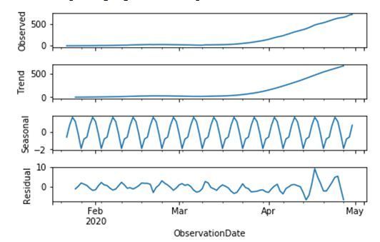
Abstract
Purpose:

Coronavirus disease is an irresistible infection caused by the respiratory disease Coronavirus 2 (SARS-
CoV-2). It was first found in Wuhan, China, in December 2019, and has since spread universally, causing a
constant pandemic. On June 3, 2020, 6.37 million cases were found in 188 countries and regions.
Prevention is the only cure for this disease. A study was carried out on Coronavirous to observe the
number of cases, deaths and recovery cases worldwide within a specific time period of five months.
Based on this data, this research paper will predict the future spread of this infectious disease in human
society.

Methods:

In our study, the data set was taken from WHO "Data WHO Coronavirus Covid-19 cases and deaths-WHO-
COVID-19-global-data". This dataset contains information about the observation date, provenance/state,
country/region and latest updates. In this article, we implemented several forecasting techniques: naive
method, simple average, moving average, single exponential smoothing, Holt linear trend method, Holt
Winter method and ARIMA, for comparison, and how these methods improve the Root mean square error
score.

Results:

The naive method is best suited as described over all other methods. In the ARIMA model, utilizing grid
search, we recognized a lot of boundaries that delivered the best-fit model for our time series data. By
continuing the model, future predictions of death cases indicate that the number of deaths will increased
by more than 600,000 by January 2020.

Conclusion:

This survey will support the government and experts in making arrangements for what is about to
happen. Based on the findings of instantaneous model, these models can be adjusted to guide long time.

Introduction
So far, Coronavirus, which has killed millions of people throughout, is constantly taking people under its
arrest. Washing hands, covering your face, isolating hygiene, and staying away from the community may
be a way to prevent this communicable disease, but it is not enough [1]. According to the WHO, there are
neither vaccinations nor equivocal antiviral medications for COVID–19 [2]. Coronaviruses are an
enormous group of infections like Middle East Respiratory Syndrome (MERS) and Severe Acute
Respiratory Syndrome (SARS) which may cause ailment in creatures or people. In people, a few

                                                 Page 2/16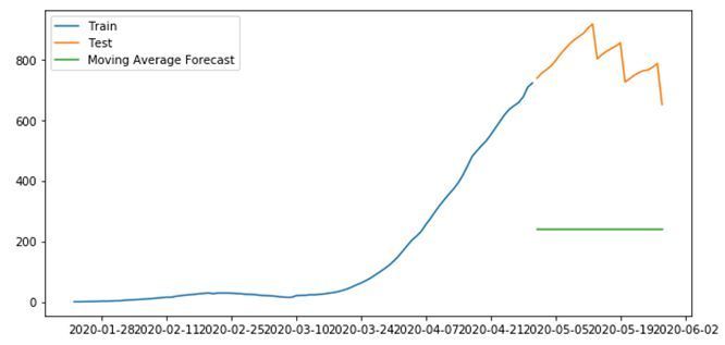
Coronaviruses are known to cause respiratory contaminations going from the basic virus to increasingly
extreme infections. The most as of late found Coronavirus causes Coronavirus infection COVID–19. The
basic symptoms for covid–19 include fever, exhaustion, brevity of breath, and failure of smell and flavor.
Further there will be progress in severe respiratory disease (ARDS), multiple organ failure, septic syncope
and blood clots. The starting of side effects is usually about 5 days; however it may be increase on or
after 2 to 14 days [3, 4, 5]. The increase of COVID–19 is mainly due to the small water droplets generated
by the contact of nearby people with others and the personal hackers who breathe contaminated
individuals, sniffing, talking or singing. Sputum and saliva spread many infections [6, 7]. Some clinical
strategies are responsible and result in the infection being transmitted more effectively than typical.

In the healthcare industry, there is a lot of evidence that machine learning algorithms can provide
effective models to solve problems in order to identify patients. To date, there is no vaccine or antibiotic
that can cure infected people and avoid this pandemic disease. Many researchers and scientists related
to machine learning are also involved in solving this situation. In order to understand the patterns and
characteristics of virus attacks, many data scientists may make the right decisions and take specific
actions.

The purpose of this study is as follows.

  1. Using time series to predict imminent deaths worldwide.
  2. Comparing the root-mean-square value of each model using time series predictive modeling through
     several methods.
  3. Finding a method suitable for prediction on the covid–19 data set.
  4. Using ARIMA model for future forecasting of death cases worldwide.

Methodology
World Health Organization (WHO) time series data has been used for experiential study. The data time is
from January 22, 2020 to May 28, 2020. Data includes confirmed cases, deaths and recovered cases
from all countries [8]. This article focuses on the data used for analysis and prediction of COVID–19 in
around the world to confirm the diagnosed patients, those who died and recovered. For analysis and
forecast quantity in patients with COVID–19 in worldwide, the following time series analysis have been
used.

We have 5 months of data (Jan 2020-May 2020) and by this statistics we will predict the figure deaths
for future.

Data Preprocessing

For creating training and test files for modeling-

                                                     Page 3/16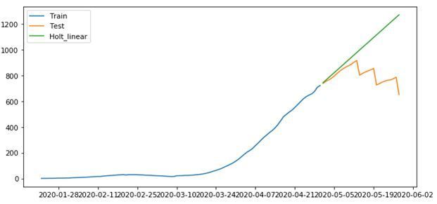
The first four months (January 2020 to April 2020) are used as training data, and the next one month
(May 2020) is used as test data.
The data set is summarized on daily basis.
The training and testing of the data set is different during the time period shown in the figure 1 below.
Naïve Method
When we use naive methods to predict the next day, we can get the value of the last day, it is estimated
that the value is the same the next day [9]. This prediction technique is called the naive method, and we
assume the subsequently predictable point is equivalent to the preceding experimental end i.e.
ŷt+1 = Ŷt
Now we will perform a naive method to predict “Death” worldwide observed in the test data set. In Figure
2 the y-axis shows the deaths of infected person and x-axis shows the time (months).
Simple Average Method
In some cases, the numbers in the data are increasing and decreasing randomly with small amplitude, the
average value is kept constant. Although the data set has a small change in the entire session, the
standard value on every occasion remains unchanged [10]. Now, we can predict the number of the
subsequent day, which is like to the standard of the precedent few days. This prediction method in which
the estimated value is the same to the standard value of the earlier experiential points is called averaging
method. We get all previously known values and evaluated standard and use it as the subsequently value
i.e.
Figure 3 is the graphical representation of given value.
Moving Average Method
In the data set, we obtained the given result multiple times, and the number of passes significantly
increased/decreased several time ranges. So as to utilize the past Average technique, we need to utilize
the mean of all the past information.
Such anticipating strategy which utilizes gap of timeframe for ascertaining the normal is called Moving
Average method [11].
Utilizing a basic moving normal form, we estimate the following significance(s) in a period arrangement
dependent on the normal of a set limited numeral p of the past qualities. Subsequently, for all i > p
Page 4/16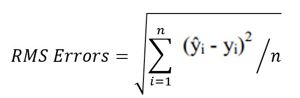
Figure 4 shows the relative measures at axis x as deaths and axis y as time.

Simple Exponential Smoothing Method

It may be sensible to affix greater loads to later discernment than to observations from the evacuated
past. The technique which takes a shot at this rule is called basic exponential smoothing [12].

Forecasts are resolved using weighted midpoints where the loads decrease exponentially as observations
begins from further previously; the smallest loads are connected with the most prepared recognition:

ŶT+1/T = αyT + α (1- α) yT–1 + α (1- α) 2yT–2 + ……

Figure 5 shows the relative measures at axis x as deaths and axis y as time.

Holt’s Linear Trend Method

We need a methodology that can portray design correctly without any assumptions. Such a system that
considers the example of the dataset is called Holt’s Linear Trend procedure [13]. Each Time plan dataset
can be broken down into its segments which are Trend, Irregularity and Residual.

We can see from the figure 6 got that this dataset follows a growing example. From now on we can use
Holt’s direct example to gauge the future pattern.

For estimating the information with pattern we need three conditions: level, pattern and consolidation of
level and pattern to find normal forecast ŷ.

Forecastŷt+h/t = lt + h bt

Level lt = αyt + (1 - α) (lt–1 + bt–1)

Trendbt = β*(lt —lt–1) + (1 - β)bt–1

In the over three conditions, we have added level and pattern to create the forecast condition.

Similarly, in the step of Figure 7, the model condition indicates that it is a weighted normal for evaluating
the model at time t, which depends on l(t)–1(t–1) and b(t–1), the past estimates value of mode.

Holt-Winters Method

Holt’s winter method is to apply exponential smoothing to the occasional segments not withstanding
level and pattern [14].

                                                     Page 5/16
Holt’s winter technique utilizes the irregularity factor. The Holt-Winters occasional strategy contains the
conjecture condition and three smoothing conditions: for the level lt, for pattern bt and for the occasional
segment meant by st with smoothing parameters α, β and γ.
Level Lt = α (yt—S t-s) + (1 - α) (Lt–1 + Bt–1)
Trendbt = β (Lt —Lt–1) + (1- β) bt–1
SeasonalS t = γ (yt - Lt) + (1- γ) S t-s
ForecastFt+k = Lt + kbt + S t+k-s
Where; s is the length of the seasonal period
0 ≤ α ≤1, 0 ≤ β ≤1 and 0 ≤ γ ≤ 1.
In figure 8, there is a level condition of weighted normal between the occasionally balanced perception at
time t and the non-accidental prediction.
Root Mean Squared Error (RMSE)
In regression line prediction, it is necessary to predict the average y value associated with a given x value
and obtain a measure of the distribution of y values around this average value. To construct the RMS
error first, we need to determine the residual error. The residual is the difference of actual value and the
predicted value [15]. The RMS error may be positive or negative because the predicted value is lower or
exceeds the actual value. Square the residuals, average the squares, and then take the square root to get
the RMS error. Then we use RMS error as a measure of the distribution of y values relative to the
predicted y values.
Where; ŷi observed value for ith observation
yi predicted value
n number of observations.
We can compare above models based on their RMSE scores in the following table 1.
Table 1: Comparison of models by RMSE values on test data
Page 6/16Model RMSE
Naïve Method 99.98448367289042
Simple Average 655.4500199405554
Moving Average 565.8570072290203
Simple Exponential smoothing 110.09483260989167
Holt’s linear Trend 277.164232654063
Holt’s Winter 236.48593103685542
ARIMA
ARIMA: Autoregressive integrated moving average, when exponential smoothing models depended on a
description of pattern and irregularity in the data; ARIMA models connect the data with one another [16].
An expansion above ARIMA is Seasonal ARIMA. This works on the irregularity of dataset simply like Holt’
winter method. The general prediction equation of ARIMA expressed by y as:
ŷt = μ + ϕ1 yt–1 +…+ ϕp yt-p - θ1et–1 -…- θqet-q
The moving average parameters (θ) are defined here so that their sign is negative in the equation. The
parameters are represented there by ar (1) and ma (1) in table 2. Stationary series may still have
autocorrelation errors, which indicates that certain the number of AR items (p≥1) and/or some MA items
(q≥1) are also required in the prediction equation.
Table 2: SARIMAX Results
coef std err z P>|z| [0.025 0.975]
ar.L1 1.9024 5.909 0.322 0.747 -9.679 13.484
ma.L1 65.0254 2.84e+04 0.002 0.998 -5.55e+04 5.56e+04
sigma2 9.1957 8028.624 0.001 0.999 -1.57e+04 1.57e+04
The coef clip shows the weight of each part (significance) and how each affects the time course of
action [17]. P> | z | this section starts with the importance of weight. Here, the p self-esteem of each
weight is lower than or close to 0.05, so it is reasonable to keep all the weights in our model.
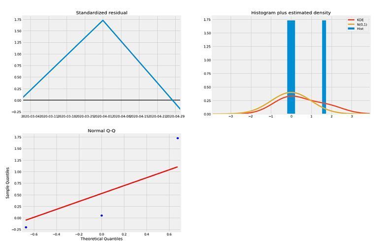
The following figure 9 produces display and examine for any unusual conduct.
Page 7/16The demonstrative model above shows that the model residuals depend on the following accompanying
ordinary conveyance:
In the histogram in addition to assessed density diagram, the red KDE line promptly follows the
N(0,1) line, which is the standard image of the ordinary dispersion with a normal estimation of 0 and
a standard deviation of 1. These shows the residuals are ordinarily distributed.
The QQ plot shows that the arranged dispersion of residuals (blue spots) follows the direct pattern of
tests taken from the standard normal distribution with N(0, 1). This strongly shows the residuals are
ordinarily dispersed.
There is no obvious seasonal variation in the standardized residuals over time; it seems to be white
noise.
In spite of the way that we have a sufficiently fit, a couple of boundaries of our seasonal ARIMA model
could be changed to improve our model fit.
Forecasting Visualization
In the last step, we portrayed in figure 10 our seasonal ARIMA time series model to forecast future values
[18].
The numbers we created (conjectures and related deterministic ranges) and related deterministic spans
can be used to additionally understand timing. Our predictions indicate that we rely on timing to maintain
a predictable rate of development.
As we further build the future, we can expect us to lose confidence in our qualities. The deterministic
extension created by our model reflects this, and as we move towards a farther future, the deterministic
span will grow larger and larger.
Discussion
The current model shows that the upcoming next few months will hard happen for the world. The control
system adopted by the different national governments is indeed very strict and works well. In addition,
adopting the direct mode can effectively supervise the recovered patients and also control the case
fatality rate. If the government does not take strict control measures to its residents, the findings of this
research may explode. The arrangement of emergency clinics and the improvement of the clinical office
should be carried out as soon as possible to establish an exponential development of the country to
prevent this from happening.
In the worldwide prediction of death cases, we used several methods to observe deaths due to the covid–
19 pandemic. The data is unstable; it also shows that the number of deaths has increased exponentially
since mid-March 2020. Another issue facing the study is Insufficient training data. 4 months (January
2020 to April 2020) data are used for training purposes, 29 days of verification data, based on which the
Page 8/16number of deaths can be determined expected in the coming months. There are very few training data for
machine learning to train itself. Moreover, the number of infected people changes rapidly, the case
occurred in mid-March.
By looking at the figure number (1–8), it is difficult to prove which method is suitable for this time series
data set in future predictions. To overcome this situation, we described the RMSE value of each method
in Table 1. Compared with other methods, the naive method has a lower RMSE score of 99.98. Therefore,
the naive method is suited in described all other methods. In the ARIMA model, utilizing grid search, we
recognized a lot of boundaries that delivered the best-fit model for our time series data. By continuing the
model, future predictions of death cases indicate that the number of deaths will increase by 500,000 to
more than 600,000 by January 2021 and beyond. But Weather conditions, national geographic
distribution, state-level residents and authority parameters may be affected the forecast. It can
supplementary develop the model prediction rate.
Conclusion
In this study, some AI models were used to decompose and predict the worldwide adjustment of COVID–
19 mortality. We investigated this information and found that the number of deaths continued to increase
from mid-March 2020. The results obtained from this inspection were taken from the information as of
May 29, 2020. In addition, according to the ARIMA model, the number of death cases will definitely
increase. Experts, welfare workers, and people who provide basic assistance types must be ensured
according to the recommended clinical standards. Due to people’s frivolous behavior, the disease spread
later, just as infected peoples can multiply the figure of cases. Maximum of fatal has not yet arrived, so
the government must be vigilant and insist on stringent measures. In addition, the arrangements for
clinical clinics across the country must be greatly improved.
In the future, it should be ensure to create computerized calculations to provide information within a
standard range and naturally predict the number of cases daily and every week. According to these
principles, the government and emergency clinics can also keep a clear responsibility and provide flexible
clinical help/services for new patients.
Declarations
Funding
This research was not funded by any agency.
Conflict of interest
The authors declare that they have no conflict of interest.
Availability of data and material
Page 9/16Dataset is available on WHO website.
Code availability
Code is available with author.
Authors' contributions
Vikas Chaurasia developed the theoretical formalism, performed the analytic calculations and performed
the analysis under the supervision of Saurabh Pal.
References
1. Nussbaumer-Streit B, Mayr V, Dobrescu AI, Chapman A, Persad E, Klerings I, et al. (April 2020).
"Quarantine alone or in combination with other public health measures to control COVID-19: a rapid
review". The Cochrane Database of Systematic Reviews. 4: CD013574
2. "Q&A on Coronaviruses (COVID-19)". World Health Organization (WHO). 17 April 2020. Archived from
the original on 14 May 2020. Retrieved 14 May 2020.
3. "Symptoms of Coronavirus". U.S. Centers for Disease Control and Prevention (CDC). 20 March 2020.
Archived from the original on 30 January 2020.
4. Hopkins C. "Loss of sense of smell as marker of COVID-19 infection". Ear, Nose and Throat surgery
body of United Kingdom. Retrieved 28 March 2020.
5. Velavan TP, Meyer CG (March 2020). "The COVID-19 epidemic". Tropical Medicine & International
Health. 25 (3): 278–280. doi:10.1111/tmi.13383. PMC 7169770. PMID 32052514.
6. Q & A on COVID-19". European Centre for Disease Prevention and Control. Retrieved 30 April 2020.
7. Hamner L, Dubbel P, Capron I, Ross A, Jordan A, Lee J, et al. (May 2020). "High SARS-CoV-2 Attack
Rate Following Exposure at a Choir Practice—Skagit County, Washington, March 2020" (PDF).
MMWR Morb. Mortal. Wkly. Rep. 69 (19): 606–610. doi:10.15585/mmwr.mm6919e6. PMID
32407303.
8. https://data.humdata.org/dataset/coronavirus-covid-19-cases-and-deaths, 2020
9. “Estimating the Shadow Economy: A ‘Naive’ Approach,” Oxford Econ. Papers, 35, pp. 23–44.
10. Genre, V., Kenny, G., Meyler, A., and Timmermann, A. (2013). Combining expert forecasts: Can
anything beat the simple average?. International Journal of Forecasting, 29(1):108 – 121.
11. Williams, P. S. Lacy, P. Yan, C.-N. Hwee, C. Liang, and C.-M. Ting, “Development and validation of a
novel method to derive central aortic systolic pressure from the radial pressure waveform using an n-
point moving average method,” J. Am. Coll. Cardiol. 57(8), 951–961 (2011).
12. Ostertagova, E. and Ostertag, O. (2012). ‘Forecasting using simple exponential smoothing’, Acta
Electrotechnica et Informatica, Vol. 12, pp. 62–66.
Page 10/1613. Yapar, S. Capar, H.T. Selamlar, I. Yavuz, Modified Holt’s Linear Trend Method, Hacettepe Univ. J. Math.
Stat. (n.d.), 2018. doi:10.15672/HJMS.2017.493.
14. Archibald, B. C., & Koehler, A. B. (2003). Normalization of seasonal factors in Winters methods.
International Journal of Forecasting, 19, 143 – 148
15. Barnston, A. G., 1992: Correspondence among the correlation, RMSE, and Heidke forecast verification
measures: Refinement of the Heidke score. Wea. Forecasting, 7, 699–709.
16. de la Torre, A. J. Conejo, and J. Contreras, “Simulating oligopolistic pool-based electricity markets: A
multiperiod approach,” IEEE Trans. Power Syst., vol. 18, no. 4, pp. 1547–1555, Nov. 2003
17. Tarsitano, A.; Amerise, I.L. Short-term load forecasting using a two-stage sarimax model. Energy
2017, 133, 108–114.
18. L. V Alquisola, D. J. A. Coronel, B. M. F. Reolope, and J. N. A. Roque, “Prediction and Visualization of
the Disaster Risks in the Philippines Using Discrete Wavelet Transform ( DWT ), Autoregressive
Integrated Moving Average ( ARIMA ), and Artificial Neural Network ( ANN ),” 2018 3rd International
Conference on Computer and Communication Systems (ICCCS), pp. 146–149, 2018
Figures
Figure 1
Distribution of training and testing dataset over time period
Page 11/16Figure 2
Naïve forecast at test dataset
Figure 3
Simple Average forecast at test dataset
Page 12/16Figure 4
Moving Average forecast at test dataset
Figure 5
Simple Exponential Smoothing forecast at test dataset
Page 13/16Figure 6
Holt's pattern to estimate the future trend
Figure 7
Holt's pattern to forecast at test dataset
Page 14/16Figure 8
Holt-Winters forecast at test dataset
Figure 9
Seasonal ARIMA diagnostics on dataset
Page 15/16Figure 10
Future values forecasts 2021 and beyond
Supplementary Files
This is a list of supplementary files associated with this preprint. Click to download.
Covid19VikasSupplymentry.docx
Page 16/16You can also read