Dbcsp: User-friendly R package for Distance-Based - arXiv
←
→
Page content transcription
If your browser does not render page correctly, please read the page content below

dbcsp: User-friendly R package for Distance-Based
                                                    Common Spacial Patterns
                                        by Itsaso Rodríguez, Itziar Irigoien, Basilio Sierra, and Concepción Arenas
arXiv:2109.00740v1 [cs.MS] 2 Sep 2021

                                                                           September 8, 2021

                                                                                  Abstract
                                               Common Spacial Patterns (CSP) is a widely used method to analyse electroen-
                                           cephalography (EEG) data, concerning the supervised classification of brain’s activity.
                                           More generally, it can be useful to distinguish between multivariate signals recorded
                                           during a time span for two different classes. CSP is based on the simultaneous diago-
                                           nalization of the average covariance matrices of signals from both classes and it allows
                                           to project the data into a low-dimensional subspace. Once data are represented in a
                                           low-dimensional subspace, a classification step must be carried out. The original CSP
                                           method is based on the Euclidean distance between signals and here, we extend it so
                                           that it can be applied on any appropriate distance for data at hand. Both, the classical
                                           CSP and the new Distance-Based CSP (DB-CSP) are implemented in an R package,
                                           called dbcsp.

                                           1     Background
                                           Eigenvalue and generalized eigenvalue problems are very relevant techniques in data
                                           analysis. The well-known Principal Component Analysis with the eigenvalue problem
                                           in its roots was already established by late seventies [Mardia et al., 1979]. In math-
                                           ematical terms, Common Spatial Patterns (CSP) is based on the generalized eigen-
                                           value decomposition or the simultaneous diagonalization of two matrices to find pro-
                                           jections in a low dimensional space. Although in algebraic terms PCA and CSP share
                                           several similarities, their main aims are different: PCA follows a non-supervised ap-
                                           proach but CSP is a two-class supervised technique. Besides, PCA is suitable for
                                           standard quantitative data arranged in a ‘individuals × variables’ tables, while CSP is
                                           designed to handle multivariate signals time series. That means that while for PCA
                                           each individual or unit is represented by a classical numerical vector, for CSP each
                                           individual is represented by several signals recorded during a time span, i.e., by a
                                           ‘number of signals × time span’ matrix. CSP allows to represent the individuals in a
                                           dimension reduced space, a crucial step given the high dimensional nature of the original
                                           data. CSP computes the average covariance matrices of signals from the two classes to
                                           yield features whose variances are optimal to discriminate the classes of measurements.

                                                                                      1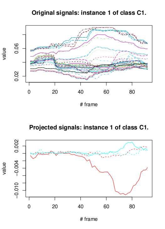
Once data is projected into a low dimensional space, a classification step is carried
out. The CSP technique was first proposed under the name Fukunaga-Koontz Trans-
form in Fukunaga and Koontz [1970] as an extension of PCA and Müller-Gerking et al.
[1999] used it to discriminate electroencephalography data (EEG) in a movement task.
Since then, it is a widely used technique to analyze EEG data and develop Brain
Computer Interfaces (BCI), with different variations and extensions [Blankertz et al.,
2007a,b, Grosse-Wentrup and Buss, 2008, Lotte and Guan, 2011, Wang et al., 2012,
Astigarraga et al., 2016, Darvish Ghanbar et al., 2021]. Samek et al. [2014] offer a
divergence-based framework including several extentions of CSP. As a general term,
CSP filter maximizes the variance of the filtered or projected EEG signals of one class
of movements while minimizing it for the signals of the other class. Similarly, it can be
used to detect epileptic activities Khalid et al. [2016] or other brain activities. Together
with, BCI systems can be of great help to people who suffer from some disorders of
cerebral palsy, or who suffer from other diseases or disabilities that prevent the normal
use of their motor skills. These systems can considerably improve the quality of life of
these people, for which small advances and changes imply big improvements. BCI sys-
tems can also contribute to the human vigilance detection, connected with occupations
involving sustained attention tasks. Among others, CSP and variations of it have been
applied to the vigilance estimation task [Yu et al., 2019].
    The original CSP method is based on the Euclidean distance between signals. How-
ever, as far as we know, it was not introduced a generalization allowing the use of any ap-
propriate distance. The aim of the present work is to introduce a novel Distance-Based
generalization of it (DB-CSP). This generalization is of great interest, since these tech-
niques can also offer good solutions in other fields where multivariate time series data
arise beyond pure electroencephalography data [Poppe, 2010, Rodríguez-Moreno et al.,
2020].
    Although CSP in its classical version is a very well-known technique in the field of
BCI, it is not implemented in R. In addition, being DB-CSP a new extension of it, it
is worth building an R package that includes both, CSP and DB-CSP techniques. The
package offers functions in a user friendly way for the less familiar users of R but it also
offers complete information in its objects so that reproducible analysis can be done, as
well as more advanced and customised analysis can be performed taking advantage of
already well-known packages of R.
    The paper is organized as follows. First, we review the mathematical formulation of
the Common Spatial Patterns method. Below, the core of our contribution, we describe
both the novel CSP’ extension based on distances and the package dbcsp. Then, the
main functions in dbcsp are introduced along with reproducible examples of their use.
Finally, some conclusions are drawn.

2     CSP and DB-CSP
Let us consider we have n statistical individuals or units classified in two classes C1
and C2 , with #C1 = n1 and #C2 = n2 . For each unit i in class Ck data from c
sources or signals are collected during T time units and therefore unit i is represented
in matrix Xik (i = 1, . . . , nk ; k = 1, 2). For instance, for electroencephalograms, data

                                             2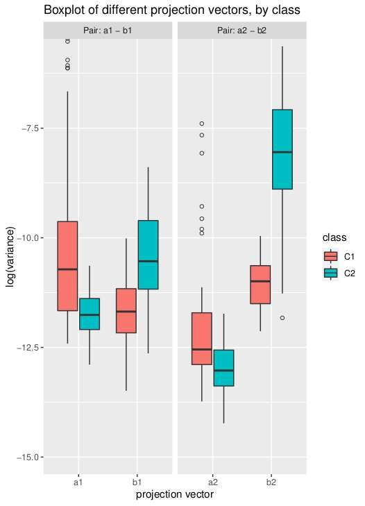
Figure 1: The flow-chart shows how the consecutive steps of filtering, feature extraction and
the construction of a classification model can be used to classify a new data.

     are recorded by a c-sensor cap each t time units (t = 1, . . . , T ). As usual, we consider
     that each Xik is already scaled or with the appropriate pre-processing in the context of
     application; for instance, if working with EGG data, each signal should be band-pass
     filtered before its use.
          The goal is to classify a new unit X in C1 or C2 . To this end, first a projection into
     a low-dimensional subspace is carried out. Then, classically the Linear Discriminant
     classifier (LDA) is applied taking as input data for the classifier the log-variance of the
     projections obtained in the first step. It is obvious that the importance of the technique
     lies mainly in the first step, and once it is done, LDA or any other classifiers could be
     applied. Based on that, we focus on how this projection into a low-dimensional space is
     done, from the classical CSP point of view as well as its novel extension DB-CSP (see
     Figure 1).

     2.0.1    Classical CSP
     The main idea is to use a linear transform to project or filter data into low-dimensional
     subspace with a projection matrix, in such a way that each row consists of weights
     for signals. This transformation maximizes the variance of two-class signal matrices.
     The method performs a simultaneous diagonalization of the covariance matrices of both
     classes. Given data X11 , . . . , Xn1 1 (matrices c × T ) from class C1 and X12 , . . . , Xn2 2
     (also matrices c × T ) from class C2 , the following steps are needed:

                                                   3
′ are the same.
• All matrices are standardized so that traces of Xik Xik
• Compute average covariance matrices:
nk
1 X ′
Bk = Xik Xik , k = 1, 2
nk
i=1
• Look for directions W = (w1 , . . . , wc ) ∈ Rc×c according to the criterion:
Maximize tr(W ′ B1 W )
subject to W ′ (B1 + B2 )W = I
The solution is given by the generalized spectral decomposition B1 w = λB2 w
choosing the first and the last q eigenvectors: WCSP = (w1 , . . . , wq , wc−q+1 , . . . , wc ).
Vectors wj offer weights so that new signals Xi1 ′ w and X ′ w have big and low
j i2 j
variability for the first q vectors (j = 1, . . . , q) respectively, and vice-versa for the last
q vectors (j = c − q + 1, . . . , c). To clarify the notation and interpretation, let us
denote aj = wj the first q vectors and bj = wc+1−j the last q. That way, and broadly
speaking, variability of elements in C1 is big when projecting on vectors aj and low on
vectors bj , and vice-versa, for elements in class C2 .
Finally, the log-variability of these new and few 2q signals are considered as input
for the classification, which classically is the Linear Discriminant Analysis. Obviously,
any other classification technique can be used.
2.0.2 Distance-based CSP
Following the commented ideas, the Distance-Based CSP (DB-CSP) is an extension of
the classical CSP method. In the same way as the classical CSP, DB-CSP gives some
weights to the original sources or signals and obtains new and few 2q signals useful
for the discrimination between the two classes. Nevertheless, the considered distance
between the signals sources can be any other than the Euclidean. The steps are the
following:
• Compute an appropriate distance measure between sources and the double-centered
inner product:
(2)
Xik → Dik → Pik = −1/2HDik H , i = 1, . . . , nk ; k = 1, 2
where H stands for the centering matrix and the superindex in brackets (2) for
squared elements in the matrix. Again, all matrices are standardized so that all
′ are the same.
traces of Xik Xik
• Compute average distance-based covariance matrices:
nk
1 X
Bk∗ = ′
Pik Pik + Xik xik 1′ + 1x′i,k Xik
′
− x′ik xik 11′
nk
i=1
where xik = 1c 1′ Xik , and k = 1, 2.
4Once we have the covariance matrices related to the chosen distance matrix, the
directions are found as in classical CSP and new signals Xik ′ a , X ′ b are built (j =
j ik j
1, . . . , q). Again, for individuals in class C1 the projections on vectors a and b are big
and low respectively; for individuals in class C2 the other way round.
It is important to note that if the chosen distance does not produce a positive
definite covariance matrix, it must be replaced by a similar one that is positive definite.
When the selected distance is the Euclidean, then, DB-CSP reduces to classical
CSP.
Once the q directions aj and bj are calculated, new 2q signals are built. Many
interesting characteristics of the new signals could be extracted, although the most
important in the procedure is the variance. Those characteristics of the new signals are
the input data for the classification step.
3 Implementation
In this section, the structure of the package and the functions implemented are ex-
plained. The dbcsp package was developed for the free statistical R environment
(http://www.r-project.org) and it is available from the Comprehensive R Archive Net-
work (CRAN) at https://cran.r-project.org/web/packages/dbcsp/index.html.
3.1 Input
The input data are the corresponding n1 and n2 matrices Xik of the n units classified
in classes C1 and C2 , respectively (i = 1, . . . , nk ; k = 1, 2). Let x1 and x2 be two
lists of length n1 and n2 , respectively, with Xik matrices (c × T ) as elements of the lists.
We also consider that new items to be classified are in list xt. The aforementioned first
step of the method is carried out by building the object called "dbcsp".
3.2 dbcsp object
The dbcsp object is an S4 class created to compute the projection vectors W . The
object has the following slots:
• Slots
X1 = "list", X2 = "list", the lists X1 and X2 (lengths n1 and n2 ) containing the
matrices Xik for the two classes C1 and C2 , respectively (i = 1, . . . , nk ; k = 1, 2).
q = "integer", to determine the number of pairs of eigenvectors aj and bj that
are kept. By default q =15.
labels = "character", vector of two strings indicating labels names, by default
names of elements in X1 and X2.
5type = "character", to set the type of distance to be considered, by default
type=’EUCL’. The supported distances are these ones:
– Included in TSdist: infnorm, ccor, sts,...
– Included in parallelDist: bhattacharyya, bray,...
mixture = "logical", logical value indicating whether to use mixture of dis-
tances or not (EUCL + other), by default mixture=FALSE.
w = "numeric", weight for the mixture of distances Dmixture = wDeuclidea +
(1 − w)Dtype , by default w=0.5.
training = "logical", logical value indicating whether to perform the classi-
fication or not. If classification = TRUE, LDA discrimination based on the
log-variances of the projected sources is considered, following the classical ap-
proach in CSP.
fold = "integer", integer value, by default fold=10. It controls the number of
partitions for the k-fold validation procedure, if the classification is done.
seed = "numeric", numeric value, by default seed=NULL. Set a seed in case you
want to be able to replicate the results.
eig.tol= "numeric", numeric value, by default eig.tol=1e-06. If the minimum
eigenvalue is below this tolerance, average covariance matrices are replaced by the
most similar matrix that is definite positive. It is done via function nearPD in
Matrix.
out= "list", list containing elements of the output. Mainly, matrix W with
vectors aj and bj in element vectors, log-variances of filtered signals in proy and
partitions considered in the k-fold approach with reproducibility purposes.
• Usage
Following the standard procedure in R, an instance of a class dbcsp is created via
the new() constructor function:
new("dbcsp", X1 = x1, X1 = x2)
Slots X1 and X2 are compulsory since they contain the original data. When a slot
is not specified, the default value is considered. First, the S4 object of class dbcsp
must be created. By default, the Euclidean distance is used, nevertheless it can
be changed. For instance, "Dynamic Transform Distance" [Giorgino et al., 2009]
can be set:
mydbcspor a mixture between this distance and the euclidean can be indicated by:
mydbcsp.mix• Arguments
object, an object of class dbcsp
vectors, integer or vector of integers, indicating the index of the projected vectors
to plot, by default index=1.
pairs logical, if TRUE the pairs aj and bj of the indicated indices are also shown,
by default pairs=TRUE.
show_log logical, if TRUE the logarithms of the variances are displayed, else the
variances, by default show_log=TRUE.
It is worthy to take into account that in the aforementioned functions, values in
argument vectors must lie between 1 and 2q, being q the number of dimensions used
to perform the DB-CSP algorithm when creating the dbcsp object. Therefore, values
1 to q correspond to vectors a1 to aq and values q + 1 to 2q correspond to vectors b1
to bq . Then, if pairs=TRUE, it is recommended that values in argument vectors are
in {1, . . . , q}, since their pairs are plotted as well. In case that values are above q, it
should be noted that they correspond to vectors b1 to bq . For instance, if q=15 and
boxplot(object, vectors=16, pairs=FALSE), vector b1 (16 − q = 1) is shown.
3.2.2 Function selectQ, Function train and Function predict
The functions in this section help the classification step in the procedure. Function
selectQ helps to find an appropriate dimension needed for the classification. Given
different values of dimensions, the accuracy related to each dimension is calculated
so that the user can assess which dimension of the reduced space can be sufficient.
A k-fold cross-validation approach or a holdout approach can be followed. Function
train performs the Linear Discriminant classification based on the log-variances of the
dimensions built in the dbcsp object. The accuracy of the classifier is computed based
on k-fold validation procedure. Finally, function predict performs the classification of
new individuals.
• Usage of selectQ
selectQ(mydbcsp)
• Arguments
object, an object of class dbcsp
Q, vector of integers which represents the dimensions to use, by default Q=c(1,2,3,5,10,15).
train_size, float between 0.0 and 1.0 representing the proportion of the data set
to include in the train split, by default train_size=0.75.
8CV, logical indicating whether a k-fold cross validation must be performed or a
hold-out approach (if TRUE, train_size is not used), by default CV=FALSE.
folds integer, number of folds to use if CV is performed.
seed numeric value, by default seed=NULL. Set a seed in case you want to be able
to replicate the results.
This functions returns the accuracies related to each dimension set in Q. If CV=TRUE,
the mean accuracy as well as the standard deviation among folds is also returned.
• Usage of train
train(mydbcsp) or embedded as a parameter in:
new(’dbcsp’, X1=x1, X2=x2, training=TRUE, type="dtw")
• Arguments
object, an object of class dbcsp
selected_q, integer value indicating the number of vectors to use when training
the model. By default all dimensions considered when creating the object dbcsp.
Besides, arguments seed and fold are available.
It is important to note that in this way a classical analysis can be carried out, in
the sense of:
• LDA is applied based on the log-variances of the dimensions indicated by the user
in, select_q;
• percentage of good classification is obtained via k-fold cross validation.
However, it is evident that it may be of interest to use other classifiers or other charac-
teristics in addition to or different from log-variances. This more advanced procedure
is explained below. See the basic analysis of the "User guide with real example" section
in order to visualize and follow the process of a first basic/classic analysis.
• Usage of predict
predict(mydbcsp, X_test=xt)
• Arguments
object, an object of class dbcsp
X_test, list of matrices for be classified.
true_targets, optional, if available, vector of true labels of the instances. Note
that they must match the name of the labels used when training the model.
94 User guide with a real example
To show an example beyond pure electroencephalography data, an Action Recognition
data is considered. Besides, in order to have a reproducible example to show the use
of the implemented functions and the results they offer, this Action Recognition data
set is included in the package. The data set contains the skeleton data extracted from
videos of people performing six different actions, recorded by a semi-humanoid robot.
It consists of a total of 272 videos with 6 action categories. There are around 45 clips
in each category, performed by 46 different people. Each instance is composed of 50
signals (xy coordinates for 25 body key points extracted using OpenPose [Cao et al.,
2019]), where each signal has 92 values, one per frame. These are the six categories
included in the data set:
1. Come: gesture for telling the robot to come to you. There are 46 instances for
this class.
2. Five: gesture of ‘high five’. There are 45 instances for this class.
3. Handshake: gesture of handshaking with the robot. There are 45 instances for
this class.
4. Hello: gesture for telling hello to the robot. There are 44 instances for this class.
5. Ignore: ignore the robot, pass by. There are 46 instances for this class.
6. Look at: stare at the robot in front of it. There are 46 instances for this class.
The data set is accessible via AR.data. Each class is a list of matrices of [K ×
num_f rames] dimensions, where K = 50 signals and num_f rames = 92 values. As
mentioned before, the 50 signals represent the xy coordinates of 25 body key points
extracted by OpenPose.
For example, two different classes can be accessed this way:
x1There are 46 instances of class C1 with [50x92] dimension.
There are 45 instances of class C2 with [50x92] dimension.
The DB-CSP method has used 15 vectors for the projection.
EUCL distance has been used.
Training has not been performed yet.
Now, if the user knows from the beginning that 3 is an appropriate dimension, the
classification step could be done while creating the object. Using classical analysis,
with for instance 10-fold, LDA as classifier and log-variances as characteristics, the
corresponding input and summary output are:
mydbcspSince the 10-fold cross-validation approach is chosen, the mean accuracies as well as
the corresponding standard deviations are returned. Thus, with Linear Discriminant
Analysis (LDA), log-variances as characteristics, it seems that dimensions related to
first and last q = 2 eigenvectors (2 × 2 dimensions in total) are enough to obtain a good
classification, with an accuracy of 90%. Nevertheless, it is also observed that variation
among folds can be relevant.
To visualize what is the representation in the reduced dimension space function
plot can be used. For instance, to visualize the first unit of the first class, based on
projections along the 2 first and last vectors (a1 , a2 and b1 , b2 ):
plot(mydbcsp, index=1, class=1, vectors=1:2)
In the top graphic of Figure 2 it can be seen what is the representation of the first
video of class C1 given by matrix X11 , where the horizontal axis represents the frames
of the video and the lines are the positions of the body key points (50 lines). In the
bottom graphic, the same video is represented in a reduced space where the video is
represented by the new signals (only 4 lines).
To have a better insight of the discriminating power of the new signals in the re-
duced dimension space, we can plot the corresponding log-variances of the new signals.
Parameter vectors in function boxplot sets which are the eigenvectors considered to
plot.
boxplot(mydbcsp, vectors=1:2)
In Figure 3 it can be seen that variability of projections on the first eigenvector
direction (log(V AR(Xik′ a ))) are big for elements in x1, but small for elements in x2.
1
Analogously, projecting on the last dimension (log(V AR(Xik ′ b ))), low variability is
1
hold in x1 and big variability in x2. The same pattern holds when projecting on vec-
tors a2 and b2 .
4.3 Basic/classic analysis new unit classification
Once the value of q has been decided and the accuracy of the classification is known, the
classifier should be built (through train()) so that the user can proceed to predict the
class a new action hold in a video belongs to, using the function predict. For instance,
with only illustrative purpose, we can classify the first 5 videos which are stored in x1.
mydbcspFigure 2: First video of class C1 represented as its original version (top) and as the projections
on vectors a1 and a2 (continuous lines) and b1 and b2 (dotted lines).
13Figure 3: Log-variabilities of the projected signals on vectors a1 and a2 and b1 and b2 and
separated by classes C1 and C2 .
14Finally notice that the user could use any other distance instead of the Euclidean between the signals to compute the important directions aj and bj . For instance, in this case it could be appropriate to use the Dynamic Time Warping distance, setting so in the argument type="dtw": # Distance DTW mydbcsp.dtw
})
})
)
return(values)
}

By means of this latter function, besides the variance of the new signals, the maximum,
the minimum, and the interquartile range can be extracted.
   Then, imagine we want to perform our classification step with the interquartile
range information besides the log-variance.

# Project units of class C1 and
projected_x1
metric = "Accuracy",
trControl = trControl)
knn_default

# Predictions and accuracies on test data
# Based on random forest classifier
pred_labels
References
Aitzol Astigarraga, Andoni Arruti, Javier Muguerza, Roberto Santana, Jose I. Mar-
  tin, and Basilio Sierra. User adapted motor-imaginary brain-computer inter-
  face by means of EEG channel selection based on estimation of distributed al-
  gorithms. Mathematical Problems in Engineering, page 1435321, 2016. URL
  https://doi.org/10.1155/2016/1435321.

Benjamin Blankertz, Motoaki Kawanabe, Ryota Tomioka, Friederike U Hohlefeld,
  Vadim V Nikulin, and Klaus-Robert Müller. Invariant common spatial patterns:
  Alleviating nonstationarities in brain-computer interfacing. In NIPS’07: Proceed-
  ings of the 20th International Conference on Neural Information Processing, pages
  113–120, 2007a.

Benjamin Blankertz, Ryota Tomioka, Steven Lemm, Motoaki Kawanabe, and
  Klaus-Robert Muller.  Optimizing spatial filters for robust EEG single-trial
  analysis.   IEEE Signal Processing Magazine, 25(1):41–56, 2007b.      URL
  https://doi.org/10.1109/MSP.2008.4408441.

Zhe Cao, Gines Hidalgo, Tomas Simon, Shih-En Wei, and Yaser Sheikh. OpenPose:
  realtime multi-person 2D pose estimation using part affinity fields. IEEE Trans-
  actions on Pattern Analysis and Machine Intelligence, 43(1):172–186, 2019. URL
  https://doi.org/10.1109/TPAMI.2019.2929257.

Khatereh Darvish Ghanbar, Tohid Yousefi Rezaii, Ali Farzamnia, and Ismail Saad.
  Correlation-based common spatial pattern (CCSP): A novel extension of csp for
  classification of motor imagery signal. PLOS ONE, 16:1–18, 2021. doi: 10.1371/
  journal.pone.0248511. URL https://doi.org/10.1371/journal.pone.0248511.

Keinosuke Fukunaga and Warren LG Koontz. Application of the Karhunen-Loève
  expansion to feature selection and ordering. IEEE Transactions on Computers, 100
  (4):311–318, 1970.

Toni Giorgino et al. Computing and visualizing dynamic time warping alignments
  in R: the dtw package. Journal of statistical Software, 31(7):1–24, 2009. URL
  http://dx.doi.org/10.18637/jss.v031.i07.

Moritz Grosse-Wentrup and Martin Buss. Multiclass common spatial patterns and in-
 formation theoretic feature extraction. IEEE Transactions on Biomedical Engineer-
 ing, 55(8):1991–2000, 2008. URL https://doi.org/10.1109/TBME.2008.921154.

Muhammad Imran Khalid, Turky Alotaiby, Saeed A. Aldosari, Saleh A. Alshe-
 beili, Majed Hamad Al-Hameed, Fida Sadeq Y. Almohammed, and Tahani S.
 Alotaibi.   Epileptic MEG spikes detection using common spatial patterns
 and linear discriminant analysis. IEEE Access, 4:4629–4634, 2016.  URL
 https://doi.org/10.1109/access.2016.2602354.

                                        18
Fabien Lotte and Cuntai Guan. Regularizing common spatial patterns to improve BCI
designs: Unified theory and new algorithms. Transactions on Biomedical Engineer-
ing, 58(2):355–362, 2011. URL https://doi.org/10.1109/TBME.2010.2082539.
Kanti V. Mardia, John T. Kent, and John M. Bibby. Multivariate Analysis. Academic
Press, London, 1979.
Johannes Müller-Gerking, Gert Pfurtscheller, and Henrik Flyvbjerg. De-
signing optimal spatial filters for single-trial EEG classification in a
movement task. Clinical Neurophysiology, 110(5):787–798, 1999. URL
https://doi.org/10.1016/S1388-2457(98)00038-8.
Ronald Poppe. Common spatial patterns for real-time classification of human actions.
In Machine Learning for Human Motion Analysis: Theory and Practice, pages 55–73.
IGI Global, 2010.
Itsaso Rodríguez-Moreno, José María Martínez-Otzeta, Basilio Sierra, Itziar Irigoien,
Igor Rodriguez-Rodriguez, and Izaro Goienetxea. Using common spatial patterns to
select relevant pixels for video activity recognition. Applied Sciences, 10(22), 2020.
URL https://www.mdpi.com/2076-3417/10/22/8075.
Wojciech Samek, Motoaki Kawanabe, and Klaus-Robert Müller. Divergence-based
framework for common spatial patterns algorithms. IEEE Reviews in Biomedical
Engineering, 7:50–72, 2014. URL https://doi.org/10.1109/RBME.2013.2290621.
Haixian Wang, Qin Tang, and Wenming Zheng. L1-norm-based common spatial pat-
terns. IEEE Transactions on Biomedical Engineering, 59(3):653–662, 2012. URL
https://doi.org/10.1109/TBME.2011.2177523.
Hongbin Yu, Hongtao Lu, Shuihua Wang, Kaijian Xia, Yizhang Jiang, and
Pengjiang Qian. A general common spatial patterns for EEG analysis with ap-
plications to vigilance detection. IEEE Access, 7:111102–111114, 2019. URL
https://doi.org/10.1109/ACCESS.2019.2934519.
19You can also read