The Optimal Parameters of Spline Regression for SNP-Set Analysis in Genome-Wide Association Study - ThaiJO
←
→
Page content transcription
If your browser does not render page correctly, please read the page content below
P-ISSN 2586-9000
                                                                                         E-ISSN 2586-9027
                       Homepage : https://tci-thaijo.org/index.php/SciTechAsia   Science & Technology Asia

                       Vol. 26 No.1 January - March 2021                                      Page: [39-52]

                                           Original research article

          The Optimal Parameters of Spline
          Regression for SNP-Set Analysis in
           Genome-Wide Association Study
              Sirikanlaya Sookkhee1, Pianpool Kirdwichai1,*, Fazil Baksh2
                   1
                   Department of Applied Statistics, Faculty of Applied Science,
       King Mongkut’s University of Technology of North Bangkok, Bangkok 10800, Thailand
               2
                 Department of Mathematics and Statistics, School of Mathematics,
                              University of Reading RG6 6AH, UK

                Received 27 March 2020; Received in revised form 9 November 2020
                  Accepted 16 November 2020; Available online 16 March 2021

ABSTRACT
       This research aims to develop a method that is capable and reliable for identifying
significant regions in Genome-Wide Association Study based on Spline regression. We
evaluate the optimal parameters in the Splines by smoothing and tuning p-values obtained
from two methods, Sequence Kernel Association Test using normal weight (SKAT normal
weight) and Generalized Higher Criticism (GHC) for testing SNP-set. False positive (FP) and
True positive (TP) rates were evaluated under different genetic models for disease with
significant thresholds adjusted for multiple hypothesis testing based on the permutation
method. The simulated data used in this research are constructed from a control data set in a
study of Crohn’s disease which is repeated 1,500 replicates for studies of size 3,000 cases and
3,000 controls. The simulation result shows that the optimal parameter in the Splines on the
 p-value of SKAT normal weight and GHC under the one disease SNP model simulation are at
the degree of freedom 1,000. GHC is shown to be preferable in terms of comparing FP and TP
rates but it is disadvantageous compared to SKAT in terms of computational burden time.
Finally, the optimal parameter of both methods was applied to real data on Crohn’s disease.
Both methods found the important regions of genes NOD2 which are strongly associated with
the development and the importance of gene NOD2 which causes Crohn’s disease.
Keywords: Sequence kernel association test; Generalized higher criticism; Permutation test;
Spline regression; B-spline; GWAS

                                                              doi: 10.14456/scitechasia.2021.5
*Corresponding author: pianpool.k@sci.kmutnb.ac.thpianpool.k@sci.kmutnb.ac.th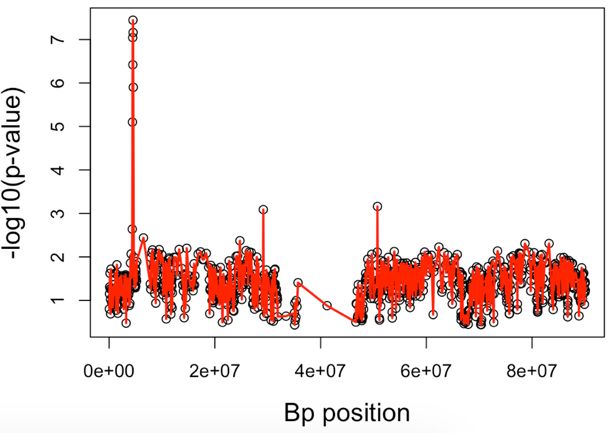
P. Kirdwichai et al. | Science & Technology Asia | Vol.26 No.1 January - March 2021

1. Introduction                                             SKAT testing models are used in this research
       A Genome-wide association study                      to find the appropriate weight. They are 1)
(GWAS) is the study of the association of                   default weight 2) Madsen and Browning
different individuals in the genetic variant                weight 3) inverse means weight, and 4)
with a phenotype. GWAS typically focuses on                 normal weight. We then compare and select
the association between the Single Nucleotide               the best method to study in the next step.
Polymorphism (SNPs) with a phenotype                               Generalized Higher Criticism (GHC)
which is the data that plays a very important               has been recently proposed for testing
role in identifying the location of DNA which               multiple SNPs in genome-wide association
causes the disease [1]. SNPs do not directly                studies. The technique uses a correlation
cause the disease, but they can indicate the                matrix to construct a new test statistic. The
risk of disease. Many diseases are still unable             GHC method is flexible to the correlation
to determine the exact gene locations that                  structure and is computationally efficient,
cause the disease. There are also hundreds of               providing a p-value without the need for the
thousands of SNPs that need to analyzed, so                 simulation of the null distribution [13].
the computational burden is another issue.                  Finally, the efficiency SKAT and GHC were
Therefore, identifying significant regions of               selected to find the region where the SNP-set
disease-gene association in high dimensional                together affects the disease by using Spline
genomewide studies is developed and                         Regression [14].
evaluated. A computationally efficient method                      In this research, a novel method that is
for obtaining the optimal tuning parameter is               capable of reducing the FP rate using spline
also evaluated using simulation.                            regression to identify the significant regions in
       The simplest and most commonly used                  the genome-wide association study is
method for analyzing SNPs and the disease is                developed and evaluated. The adjusting
a single SNP analysis that can identify SNPs                 p-value using b-spline with the cubic function
that cause the disease by analyzing only one                that gives optimal smoothing and tuning
location at a time. It is the traditional testing           parameters is considered.
method that has been considered as the                             Another important aspect of GWAS is
approach for genetic association analysis [2-               the     testing     of     many      hypotheses
3]. However, the results of the single-SNP                  simultaneously, resulting in high false
analysis are not sufficiently informative to                positives and incorrectly ascribing scientific
interpret without explicit references to linkage            significance to a statistical test [15].
disequilibrium (LD) patterns of candidate                   Bonferroni adjustment is a popular method for
variants [4]. Many studies have discovered                  controlling the probability of the type I error.
that SNPs that cause the disease can be                     However this approach tends to be highly
located at the same chromosome [5-7]. The                   constringent and conservative [16-17].
Sequence Kernel Association Test (SKAT)                     Therefore, the permutation method was
was proposed to analyze the association                     selected as the alternative way of controlling
between SNP-set with disease outcome under                  the type I error rate which is based on the
a logistic kernel machine model. This method                nonparametric method. It is a good choice for
aggregates individual SNP score statistics in               the hypothesis test of unknown distribution.
the SNP set and efficiently compute SNP-set                 This approach will be estimating the sampling
level p-values [8]. SKAT is a supervised and                distribution of a test statistic under the null
flexible computationally efficient regression               hypothesis that a set of genetic variants does
method to test for the association between                  not affect the outcome. In this research,
common or rare variants and disease [9-12].                 10,000 replicates were used to compute the
SKAT performance depends on weight                          multivariate sampling distribution under the
configuration. Therefore, varying weights of                null hypothesis with no gene effect. This

                                                       40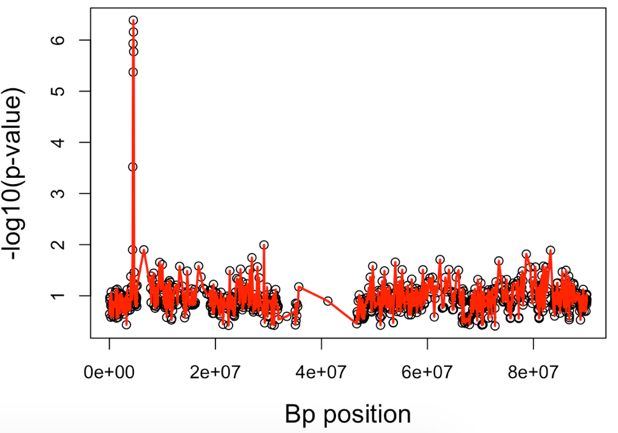
P. Kirdwichai et al. | Science & Technology Asia | Vol.26 No.1 January - March 2021
X − j ,X j
( X − ) = 0
approach provides a highly reliable
distribution and gives the exact p-value of the j .
test statistics [18-19]. The genotype data [20] ,otherwise
was used in this simulation study from 1,504
individuals in the 1958 British Birth Cohort on A(X) is the spline function of degree
Chromosome 16 which is being associated m. b j is the associated spline coefficient
with Crohn's disease. But It is not clear that with k knots and there are k+1 polynomial
which SNPs or genes are responsible for this of degree m. X j is the set of basis function
disease.
and is the coefficients for the polynomial
Therefore, the objective of this research
is to find the optimal parameters of b-spline to [22].
identify the significant SNP-set from the The most popular spline is the cubic
SKAT and GHC methods. True positive (TP) spline
k
and false positive (FP) rates use the A(X) = b0 + b1X + b 2X 2 + b3X3 + j (X - j )3. (2)
permutation threshold as considered to find j =1
the efficiency method. Finally, the optimal A much better representation of
parameters of both methods were selected to splines for computation is as linear
apply to the real data from the WTCCC study combinations of a set of basis splines called
on Crohn’s disease [20]. Basis splines (B-spline) which are non-zero
over a limited range of knots. A B-spline is
2. Methods a curve created from sub-curves in each
This section will present the Spline range that can change the coefficient of the
Regression which was selected to identify control point, which will affect the shape of
the gene regions. The permutation method the curve only near the control point. This
was selected for finding the appropriate makes the B-spline curves easy to shape and
thresholds of the theoretical SKAT and does not affect the overall curve. These sub-
GHC methods. curves are created using the n polynomial.
The value of n affects the smoothness of the
2.1 Spline regression
curves. The basic properties of B-spline
A spline [21] is a piece-wise
polynomial with the piece defined by a throughout this work, let r1, r2 ,..., rk be the
sequence of knots in the range of X order of knots included in a real interval
[a, b] . A spline of order p ≥ 0 is a piecewise
1 2 k , polynomial function of order p such that its
derivatives up to order p-1 are continuous at
such that the pieces join smoothly at every knot r1, r2 ,..., rk . The set of splines order
the knots. For a spline of degree m, one
usually requires the polynomial and their p over the knots r = r1 , r2 ,..., rk is a vector
first m-1 derivatives to agree at the knots, so space of dimension p + k + 1.
that m-1 derivatives are continuous. A A spline basis is the truncated power
spline of degree m can be represented as: basis: {x 0 , x1,..., x p ,(x - r1 )p ,...,(x - rk )p }. Reference
m k
[23] introduced B-spline as more adapted to
A(X) = b jX j + j (X - j ) m , (1) computational implementation of spline
j= 0 j=1 regression.
B-spline is a spline with a non-zero
where the notation over [x k , x p+k+1 ] for some k. For
41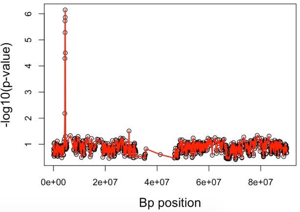
P. Kirdwichai et al. | Science & Technology Asia | Vol.26 No.1 January - March 2021
i = 1, 2,..., p + k + 1 , the i - th B-spline of 0.05. We use linear interpolation for finding
order p is noted N i,p (x) and defined by the thresholds
2.3 SNP-set methods
x - ri ri+p+1 - x The Sequence Kernel Association
N i,p (x) = N i,p-1 (x) + N i+1,p-1 (x). (3)
ri+p - ri ri+p+1 - ri+1 Test or SKAT [17] is the test for the joint
effects of multiple variants in a region of the
In this research, a B-spline was genome on the disease which the regions
selected fitting the p-value which uses a were defined by genes. P-values were
function in R for calculating the basis. calculated for an association underlying the
Therefore, the main problem was finding test procedure that can be viewed within the
the optimal parameter of bs function in R. kernel machine regression framework [9,
The parameter of bs() function is bs(x, df = 25]. The semiparametric logistic regression
null, knots = null, degree = 3) where x is a model was used in the feature of SKAT
predictor, df is degree of freedom, knots are including the parametric and nonparametric
the internal breakpoints to set the default functions component effect the conditional
which based on quantile of x and degree of probability of a dichotomous outcome [26].
3 which is the cubic spline. We compute B- The semiparametric logistic regression
spline coefficients for regression quantile B- model for the i th individual is
spline with fixed knots and specify the df.
The optimal df can be obtained from tuning logitP(yi = 1) = 0 + α ' Ci + h(Ti ), (4)
which will specify the df value in one
hundred increments in the range of 100 - where y i is a binary disease outcome taking
900.
values 0 (no disease) or 1 (disease) where
2.2 Permutation method i = 1, 2, …, n , α 0 is an intercept term, is
A permutation method (also called a the vector of regression coefficients for the
randomization test, re-randomization test, or covariates C i and Ti are the observed
an exact test) is a nonparametric method for variants and are related to disease through a
estimating the sampling distribution of a test nonparametric function h() , which is
statistic under the null hypothesis that a set assumed to lie in a functional space
of genetic variants has no effect on the generated by a positive semidefinite kernel
outcome. This approach provides a highly
function K(,) [17]. H 0 : h(T) = 0 is the
reliable distribution of the test statistic but
requires many samples generated under the null hypothesis of no association between
null model. If the labels are exchangeable the disease and gene region which were
under the null hypothesis, then the resulting tested by assuming that the n 1 vector
tests yield exact significance levels [18]. A h = [h(T1 ),..., h(Tn )] for the genetic effects
permutation test is a good choice for of the n subjects follows a distribution with
hypothesis test of unknown distribution. It mean 0 and covariance K , where is a
works regardless of the shape and size of the variance component. The semiparametric
population to give the exact p-value [24]. In logistic regression model [10] is equivalent
this research, we use 10,000 replicates for to
computing the multivariate sampling
distribution under the null hypothesis with (5)
no gene effect and to establish significance
thresholds giving a Type I error close to
42P. Kirdwichai et al. | Science & Technology Asia | Vol.26 No.1 January - March 2021
where is a vector of where B denotes the beta function, a and b
are prespecified scale and shape parameters
regression coefficients for the p observed
and x j is the estimated minor allele
variants in the gene region with each b j
frequency (MAF) for SNP j using all cases
following an arbitrary distribution with
mean of 0 and a variance of where and controls. Four weights were considered
which are default, Madsen and Browning,
w j is a pre-specified weight for variant j inverse mean and normal weight.
and is the variance component. The null The default weight chooses a small a
hypothesis is equivalent to the and large b as Beta(x j :1,25) which
substantially up-regulates rare variants and
hypothesis which may be tested
down-regulates common variants [10]. The
with a variance-component score test statistic Madsen and Browning weight was defined
as Beta(x j : 0.5,0.5) , which corresponds to
S = (Y − ˆ )K (Y − ˆ ), (6)
w j = 1/ MAFj (1- MAFj ) ; that is w j is the
where K = TWT , is the predicted mean inverse of the variance of the genotype
of Y = (y1 ,…, yn )¢ under H 0 that is marker j. The inverse mean is equivalent to
, and are Beta(x j : 0.5,1) the weight based on function
estimated under the null model by w j = 1/ x j . The normal weight is
regressing y on the covariate C and
Beta(x j :10,10) which gives the appearance
T = [T1 ,...,Tn ] is an n p matrix with
of a symmetrical distribution similar to the
elements variant j of individual i , and normal distribution [17].
W = diag(w1 , ..., w p ) contains the weights
Generalized Higher Criticism or
of the p variants. SKAT uses the variance- GHC [13,17] is the method for testing
component score test statistic to test the null associated gene regions by using single
of no genetic effect but exploits the variant statistics and their correlation matrix
semiparametric regression approach in to construct a new test statistic and its
computing K . The form for K used by distribution. Considering the
SKAT is an n n symmetric matrix with parametrization of P(yi = 1) for the j- th
elements K(Ti ,Ti¢ ) that measures genetic variant in a set of p variants,
similarity between the i - th and i - th
subjects in the study. The weighted linear logit P(yi = 1) = 0 + Ci + ji, j , (8)
p
kernel K (Ti , Ti ) = w ijTi Ti was selected
j=1
in this paper. Weight functions can be where b j is the effect of the j- th variant
specified in the SKAT package in R which
and Ti, j is the observed j- th variant with
are based on the Beta density function
Beta(x j : a,b) the i - th subject, and the other terms are as
in the previous section. The GHC approach
exploits the fact that while p might be large
x ja-1 (1- x j )b-1
wj = ,0 < x j < 1; a, b > 0, (7) in the test of the global null , in a
B(a,b)
genetic construct variants are likely to be
correlated and generally only a small subset
43P. Kirdwichai et al. | Science & Technology Asia | Vol.26 No.1 January - March 2021
of variants are signals for association. In P(GHC) ≥ TGHC (13)
other words, a sparse set of the
is not zero. GHC aims to is also calculated accounting the correlation.
The algorithm behind both methods is
account for both sparse signals and implemented in the R packages SKAT [8]
correlation among SNPs when combining and GHC [27], respectively.
individual marker test statistics.
Let Tj = (T1, j ,..., Tn , j ) be the vector of
3. The Data and Model Simulation
observed variants at the j-th marker,
The genotype data used in this
Y = (y1 ,…, yn ) be the observed disease
simulation are the SNPs on Chromosome 16
status and ˆ = (ˆ 1 , ˆ n ) be the from 1,504 unaffected individuals in the
predicted mean for Y under the assumption WTCCC study of Crohn's disease. The 13,
of no genetic effect. The statistical the 479 SNPs from each individual are used to
score for j , is under the global null construct two haplotypes to give a total of
3,008 haplotypes for use in the simulation
study. The simulation is repeated 1,500
Tj' (Y − ˆ ) times for a study size of 3,000 cases and
Zj = , (9)
Tj' PTj 3,000 controls.
The new genotype data were
generated and assigned disease status based
of P = W − WC(CWC) −1 Cw and on two disease SNPs. The first SNP
W = diag ˆ 1 (1 − ˆ 1 ), , ˆ n (1 − ˆ n ) . These rs3789038 is located at position
individual variants test the statistics of 50711672bp in gene HMOX2 and has MAF
asymptotically jointly distributed as equal to 0.31. The second, SNP rs3785142
has MAF equal 0.48 and is located at
where the (i,k) th position 50753236bp in gene CYLD. There
component of is estimated by is a total of 7 SNPs in the data on gene
HMOX2 with pairwise correlation ranging
between 0.93 and 0.99, with median 0.99,
(10) while there are 8 SNPs in the data on CYLD
having pairwise correlations between 0.51
and 0.99, with the median equal to 0.93.
Define S(t) by [17].
The model for one disease SNP used
p
S(t) = 1{|z j | t} . (11) to generate disease status is
j=1
The generalized higher criticism test e0 +1T
P(diseased | T) = , (14)
statistic, defined as 1 + e0 +1T
(12) where T is the number of copies of the rare
allele of the disease SNP, 0 is a pre-
specified baseline relative risk of disease
where is the standard normal and 1 is the gene effect. In this study, 0.1,
distribution function and , 0.2, 0.4 and 0.7 are arbitrarily chosen for
calculated by accounting for the correlation gene effect of 1 and we found that small
between the Zjs . The p-value gene effects are able to classify rare variants
44P. Kirdwichai et al. | Science & Technology Asia | Vol.26 No.1 January - March 2021
better than large gene effects. Therefore, we are then used to construct the genotype of an
have chosen the gene effect equal to 0.2. individual in the study. The disease status
The disease model for two disease (y = 0,1) is determined using the probability
SNPs is from the logistic regression in Equation 5
and 6, respectively. The cases and controls
e0 +1T1 +2 T2 are generated under the randomly selected
P(diseased | T1 , T2 ) = . (15)
1 + e0 +1T1 +2 T2 assumption and disease SNP are rs3789038
and rs3785142.
This model assumes the two disease Determining the status of an
SNPs act linearly on the logit scale and two individual is performed by considering
situations are investigated. The first is for random numbers from the uniform
gene effect 1 = 0.1 and 2 = 0.2 while in distribution to compare with the probability.
If the probability value is more than the
the second case the gene effects are fixed at
random numbers, we define as case (disease
1 = 0.2 and 2 = 0.1. Once again small
= 1) and control otherwise (no disease = 0).
gene effects for 1 and 2 give a better The SNPs are coded in three fashions, with
result in classifying rare variants. The 0, 1, and 2 corresponding to homozygotes
example genotype data in simulation were for the major allele, heterozygotes, and
shown in Table 1. The haplotypes are next homozygotes for the minor allele,
coded to 0 (major allele) and 1 (minor respectively. The genotype data from
allele) and used to construct pairs of generating simulated data is shown in Table
parental genotypes using randomly selected 1.
haplotypes. Each pair of parental genotypes
Table 1. The genotype data from generating simulated data 3,000 cases and 3,000 controls.
Individual Disease status SNP1 SNP2 SNP13,479
1 1 0 1 2 2
2 1 2 1 1 1
1
3000 1 0 0 1 1
3001 0 2 1 1 1
3002 0 0 1 1 0
0
6000 0 0 0 0 1
4. Simulation Study
In this research we considered the #significant SNP except disease SNP
FP = . (16)
efficiency of the model by using the false # Atotal SNPs # Atotalreplicates
positive (FP) and true positive (TP) rates. #significant SNP in disease SNP
TP = . (17)
The FP is the number of disease SNPs or #A total replicates
SNP-set that are not identified, whereas the
TP is the number of times the disease SNPs
were detected. The result in this research are In this research, we present the
based on 1,500 replicates. The equation for simulation result of SKAT and GHC with
calculating FP and TP rates in the study are B-spline for two cases, one disease SNP
as follows: case and two disease SNPs case.
45P. Kirdwichai et al. | Science & Technology Asia | Vol.26 No.1 January - March 2021
Case I: One disease SNP increases FP and TP rates are decreasing. In
The FP and TP rates of SKAT normal this case, both methods were confirmed by
and GHC of rs3789038 and rs3785142 as the simulation results which show that b-
disease SNP with gene effect size 1 = 0.2 spline under the degree of freedom 1,000
are provided in Table 2. The result has which is the optimal parameter with the
shown that when the degree of freedom lowest FP and high TP.
Table 2. The FP and TP rates from SKAT normal and GHC with B-spline based on
permutation threshold with rs3789038 and rs3785142 as disease SNP and effect size b1 = 0.2
Disease SNP rs3789038 Disease SNP rs3785142
d.f.
SKAT normal GHC SKAT normal GHC
FP TP FP TP FP TP FP TP
400 0.01505 0.95 0.00860 0.91 0.01440 0.50 0.01271 0.58
500 0.01082 0.93 0.00784 0.88 0.01124 0.60 0.01049 0.60
600 0.01152 0.88 0.00703 0.86 0.01003 0.70 0.00861 0.60
700 0.01087 0.86 0.00668 0.83 0.00925 0.74 0.00791 0.61
800 0.01030 0.85 0.00728 0.83 0.00846 0.78 0.00740 0.62
900 0.00963 0.86 0.00616 0.81 0.00782 0.80 0.00684 0.62
1000 0.00953 0.86 0.00616 0.81 0.00771 0.79 0.00679 0.62
1100 0.00953 0.86 0.00616 0.81 0.00771 0.79 0.00679 0.62
1200 0.00953 0.86 0.00615 0.81 0.00771 0.79 0.00679 0.62
Table 3. The TP and FP rates of SKAT normal and GHC method with B-spline based on
permutation threshold with rs3789038 and rs3785142 as disease SNP.
d.f.
2 = 0.2 and 1 = 0.1 1 = 0.1 and 2 = 0.2
SKAT normal GHC SKAT normal GHC
FP TP FP TP FP TP FP TP
400 0.07079 0.99 0.03029 0.95 0.08264 0.88 0.03595 0.85
500 0.05783 0.98 0.02557 0.94 0.06972 0.88 0.02970 0.85
600 0.05165 0.97 0.02169 0.93 0.06147 0.91 0.02427 0.85
700 0.04779 0.96 0.02002 0.93 0.05660 0.91 0.02202 0.85
800 0.04483 0.95 0.01909 0.92 0.05273 0.92 0.02053 0.85
900 0.04224 0.96 0.01808 0.91 0.04953 0.94 0.01908 0.85
1000 0.04180 0.95 0.01796 0.91 0.04901 0.93 0.01900 0.85
1100 0.04180 0.95 0.01796 0.91 0.04901 0.93 0.01900 0.85
1200 0.04180 0.95 0.01796 0.91 0.04901 0.93 0.01900 0.85
The FP rate of SKAT normal is seen comes at a higher TP rate 0.79. The FP rate
at 0.00953 to be higher than GHC but this of the GHC is 0.00679 and the TP rate is
comes at a higher TP rate 0.86. The FP rate 0.62, which show that there is a small
of the GHC is 0.00616 and the TP rate is difference in FP while much higher TP.
0.81 show that there is a small degree of
Case II: Two disease SNPs
difference in the FP and TP.
Comparisons of the FP and TP rates
In the case of rs3785142 as disease
of SKAT normal and GHC of rs3789038
SNP, the result has shown that when the
and rs3785142 under the disease model for
degree of freedom increases FP and TP rates
two disease SNP are shown in Table 3. The
are roughly increasing. The simulation
FP and TP rates for SKAT normal and GHC
results show b-spline under the degree of
with a gene effect sizes of 2 = 0.2 and 1 =
freedom 1,000 which is the optimal
parameter with the lowest FP and high TP. 0.1. This is consistent with the finding in
The FP rate of SKAT normal is seen at Table 2. The simulation results show that b-
0.00771 to be higher than GHC but this spline under the degree of freedom 1,000 is
46P. Kirdwichai et al. | Science & Technology Asia | Vol.26 No.1 January - March 2021
the optimal parameter with the lowest FP. 0.04901 to be higher than GHC but this
The FP rate of SKAT normal is seen at comes as higher than the TP rate of 0.93.
0.04180 to be higher than GHC but this The FP rate of the GHC is 0.01900 and the
comes at a higher TP rate of 0.95. The FP TP rate is 0.85 showings an above moderate
rate of the GHC is 0.01796 and the TP rate difference in FP and TP.
is 0.91. The finding confirmed that the GHC
In the case of the gene effect size 1 = outperforms SKAT normal. The different
0.1 and 2 = 0.2, the result has shown that disease SNP affects the efficiency of the
model which is SNP rs3789038 is driving
when the degree of freedom increases, FP
the disease gene relationship in the
and TP rates are increasing. The simulation
simulation model. The ROC curves of the
results show that b-spline under the degree
disease model for one disease SNP are
of freedom 1,000 which is the optimal
shown in Fig. 1 and Fig. 2 and two disease
parameter with the lowest FP and a high TP.
SNP in Fig. 3 and Fig. 4, respectively.
The FP rate of SKAT normal is seen at
Fig. 1. The ROC curve for FP and TP rates from SKAT and GHC with B-spline with rs3789038 as
disease SNP and effect size 1 = 0.2
Fig. 2. The ROC curve for FP and TP rates from SKAT and GHC methods using B-spline with
rs3785142 as disease SNPs and effect size 1 = 0.2
47P. Kirdwichai et al. | Science & Technology Asia | Vol.26 No.1 January - March 2021
Fig. 3. The ROC curve for FP and TP rates from SKAT and GHC method using B-spline with
rs3789038 and rs3785142 as disease SNP and respective effect sizes of 2 = 0.2 and 1 = 0.1
Fig. 4. The ROC curve for FP and TP rates from SKAT and GHC method using B-spline with
rs3789038 and rs3785142 as disease SNP and respective effect sizes of 1 = 0.1 and 2 = 0.2
The result shows that SKAT and the significance of SKAT normal (a) and
GHC give a comparable result. The optimal GHC (b) with degree of freedom 1,000 for
degree of freedom of both methods is 1,000. one and two disease SNPs genetic models
The example of the B-spline for declaring are shown in Fig. 5 and Fig. 6, respectively.
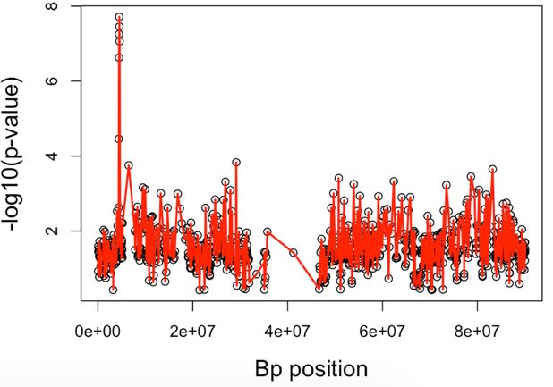
48P. Kirdwichai et al. | Science & Technology Asia | Vol.26 No.1 January - March 2021
(a) (b)
Fig. 5. The horizontal line of permutation threshold for declaring significant of SKAT normal (a) and
GHC (b) with B-spline df 1,000 for one disease SNP genetic model.
(a) (b)
Fig. 6. The horizontal line of permutation threshold for declaring significant of SKAT normal (a) and
GHC (b) with B-spline df 1,000 for two disease SNP genetic model.
5. Real Data Application 12 SNPs were located in NOD2, and 8
Both methods that were evaluated in SNPs were located in CLDY gene,
the previous section can be applied to real respectively. Other significant genes were
data to define the location of SNP or the LOC646828, intron gene 89 and SMG1P5.
region that causes the disease. The data set Moreover, the GHC method found four
used has 13,479 SNPs on Chromosome 16 regions, the largest region is called region 7
which comprise 2,005 cases and 1,500 located at 114,090 basepairs and contains a
controls of Crohn’s disease studies. Table 4 cluster 27 SNPs. There are 7 SNPs located
shows the SNPs which are declared as within an intron (a region inside a gene), 12
significant by SKAT normal and GHC with SNPs located in NOD2 and 8 SNPs located
B-spline. SKAT normal found four regions. in the CLDY gene, respectively. Other
The largest region called region 7 located at significant genes were SMG1P5,
114,090 basepairs and contains a cluster of LINC01566, and intron gene 173.
27 SNPs. There are 7 SNPs located within The result obtained from the real
an intron gene 174 (a region inside a gene), data shows that both methods give the same
49P. Kirdwichai et al. | Science & Technology Asia | Vol.26 No.1 January - March 2021
regions that cause the disease. Especially, lower FP in the simulation studies. In
both methods were finding gene NOD2 addition, GHC has an advantage in terms of
which declared to concern Crohn’s disease lower computational cost. Therefore, it is
[28-30]. However, when comparing the clearly seen that GHC with B-spline is
performance, all GHC with B-spline give a preferable.
Table 4. Gene on Chromosome 16 declared as significant SKAT and GHC method without
and with B-spline for the WTCCC study of Crohn’s disease.
Region SKAT normal with B-spline GHC with B-spline
1 LOC646828, Intron Gene 89 -
2 - -
3 SMG1P5 SMG1P5
4 - LINC01566
5 Intron Gene 151, KIF18BP1 -
6 - Intron Gene 173
7 Intron Gene 174, NOD2, CYLD Intron Gene 174, NOD2, CYLD
6. Discussion and Conclusion obtaining the SKAT and GHC p-value, it
Identifying an optimal parameter and was found that the GHC takes the most time
appropriate thresholds for declaring to analyze, about 750 hours while SKAT
significance are two important and related normally used only about 100 hours. It is
problems remaining to be solved. It is clear that SKAT normal is very
desirable to have an optimal parameter. The advantageous and can reduce computational
findings showed that b-spline under the time while efficiency is the same as GHC.
degree of freedom 1,000 is the optimal In the section of real data analysis, it
parameter for all conditions. Obviously, was found that both methods found
when setting the degree of freedom more particularly important regions. Region 4 was
than 1,000 the FP and TP rates are involved in genes 174, NOD2 and CYLD.
unvarying. Defining the degree of freedom Many researchers found that gene NOD2 is
over the number of variables (SNP-sets) strongly associated with the development
causes the B-spline to overfit with the data and important genetic variant cause Crohn’s
set. Moreover, if we are increasing the disease [28-30]. Finally, the researchers
degree of freedom it will take a lot of time expect that this method will be able to apply
to fit the B-spline. If we compared the to other diseases that have not yet been able
efficiency of the model using FP and TP to identify the SNP-sets that affect the
rates, SKAT normal is highly TP and FP disease.
while GHC with B-spline is less than TP
and gives the lower FP. Both methods have References
different advantages and disadvantages, [1] Bush WS, Moore JH. Genome-wide
SKAT normal gives a high FP while GHC association studies. PLoS Comput. Biol
gives the lower FP which we focus on 2012; 8: e1002822.
reducing. But it is difficult to specify the
efficiency of the model. It can be seen that [2] Lewis CM. Genetic association studies:
both models obtain the same region in real design, analysis and interpretation.
data application analysis. There are many Briefings in Bioinformatics 2002; 3: 146-
factors that should be considered as well, 53.
such as the computation. In the process of
50P. Kirdwichai et al. | Science & Technology Asia | Vol.26 No.1 January - March 2021
[3] Clarke GM, Anderson CA, Pettersson approach for rare-variant association
FH, Cardon LR, Morris AP, Zondervan testing with application to small-sample
KT. Basic statistical analysis in genetic case-control whole-exome sequencing
case-control studies. Nature Protocols studies. American Journal of Human
2011; 6: 121–33. Genetics 2012; 91: 224-37.
[4] Lee Y, Luca F, Pique-Regi R, Wen X. [12] Ionita-Laza I, Lee S, Makarov V, Buxbaum
Bayesian multi-SNP genetic association JD, Lin X. Sequence kernel association
analysis: control of FDR and use of tests for the combined effect of rare and
summary Statistics. bioRxiv 2018; common variants. American Journal of
316471. Human Genetics 2013; 92: 841-53.
[5] Schaid DJ, Rowland CM, Tines DE, [13] Barnett I, Mukherjee R, Lin X. The
Jacobson RM, Poland GA. Score tests for Generalized higher criticism for testing
association between traits and haplotypes SNP-set effects in genetic association
when linkage phase is ambiguous. studies. Journal of the American Statistical
American Journal of Human Genetics Association 2017; 112: 64-76.
2001; 70: 425-34.
[14] Goepp V, Bouaziz O, Nuel Z. Spline
[6] Zhao Y, Chen F, Zhai R, Lin X, Diao N, regression with automatic knot selection.
Chritiani DC. Association Test Based on HAL Archives-Ouvertes.fr 2018: hal-
SNP Set: Logistic Kernel Machine Based 01853459.
Test vs. Principal Component Analysis.
PLoS ONE 2012; 7: 1-11. [15] Johnson RC, Nelson GW, Troyer JL,
Lautenberger JA, Kessing BD, Winkler
[7] Kirdwichai P, Baksh MF. The analysis of CA, O’Brein SJ. Accounting for multiple
genomewide SNP data using comparisons in a genome-wide association
nonparametric and kernel machine study (GWAS). BMC Genomics 2010; 11:
regression. Journal of Applied Science 724.
2019; 18: 20-30.
[16] Zeng P, Zhao Y, Qian C, Zhang L, Zhang
[8] SKAT package [Internet]. [cited 2019 Nov R, Gou J, Liu J, Liu L, Chen F. Statistical
10]. Available from: https://cran.r- analysis for genome-wide association
project.org/web/packages/SKAT/SKAT.pdf study. The Journal of Biomedical
Research 2015; 29: 285-297.
[9] Wu MC, Kraft P, Epstein MP, Taylor D,
M, Chanock SJ, Hunter DJ, Lin X. [17] Sookkhee S, Baksh MF, Kirdwichai P.
Powerful SNP-set analysis for case- Efficiency of Single SNP analysis and
control genome-wide association Sequence Kernel Association Test in
studies. American Journal of Human Genome-wide Association Analysis. In:
Genetics 2010; 86: 929-42. Ao SI, Castillo O, Douglas C, Dagan DF,
Korsunsky AM, eds. Proceedings of the
[10] Wu MC, Lee S, Cai T, Li Y, Boehnke M, International MultiConference of
Lin X. Rare-variant association testing Engineers and Computer Scientists; 2018
for sequencing data with the sequence Mar 14-16; Hong Kong. IAENG
kernel association test. American Journal International Journal of Applied
of Human Genetics 2011; 89: 82-93. Mathematics. [cited 2019 Nov 9].
Available form:
[11] Lee S, Emond MJ, Bamshad MJ, Barnes http://www.iaeng.org/publication/IMECS
KC, Rieder MJ, Nickerson DA, NHLBI 2018/IMECS2018_pp308-313.pdf
GO Exome Sequencing Project—ESP
Lung Project Team, Christiani DC, [18] Corcoran CD, Senchaudhuri P, Mehta
Wurfel MM, Lin X. Optimal unified CR, Patel NR. (2005). Exact Inference for
51P. Kirdwichai et al. | Science & Technology Asia | Vol.26 No.1 January - March 2021
Categorical Data. In Armitage P, Colton [25] Lettre G, Lange C, Hirschhorn JN. Genetic
T, eds. Encyclopedia of Biostatistics (2nd model testing and statistical power in
ed.) pp.1804-1820. Chichester, UK: John population-based association studies of
Wiley. quantitative traits. Genet Epidemiol 2007;
31: 358-362.
[19] Permutation Test & Monte Carlo
Sampling [Internet]. [cited 2019 Jan 10]. [26] Banerjee M, Mukherjee D, Mishra S.
Available from : Semiparametric binary regression models
http://www.let.rug.nl/nerbonne/teach/rema- under shape constraints. Research
stats-meth- supported in part by National Science
seminar/presentations/Permutation/Permuta Foundation grants. [Internet]. [cited 4 Nov
tion-Monte-Carlo-Jianqiang-2009.pdf 2020]. Available from :
http://dept.stat.lsa.umich.edu/~moulib/bmm
[20] The Wellcome Trust Case-Control techrep.pdf
Consortium. Genome-wide association
study of 14,000 cases of seven common [27] Barnett I. GHC: Computes P-values for
diseases and 3,000 shared controls. Nature the Generalized Higher Criticism. R
2007; 447: 661-678. package version 1.0. [Internet]. [cited 2019
Jan 10]. Available from:
[21] Rodríguez G. Logit Models for Binary https://scholar.harvard.edu/ibarnett/software
Data. [Internet]. [cited January 10, /generalized-higher-criticism
2019]. Available from :
https://data.princeton.edu/wws509/notes/c3. [28] Michail S, Bultron G, DePaolo RW.
pdf Genetic variants associated with Crohn’s
disease. The Application of Clinical
[22] Perperoglou A, Sauerbrei W, Genetics 2013; 6: 25–32.
Abrahamowicz M, Schmid M. A review of
Spline function procedures in R. BMC [29] Sidiq T, Yoshihama S, Downs I,
Medical Research Methodology 2019; Kobayashi KS. Nod2: A Critical Regulator
19:1-16. of ileal Microbiota and Crohn’s Disease.
Frontiers in Immunology 2016; 7: 1-11.
[23] De Boore C. A Practical Guide to Splines.
New York: Springer-Verlagp; 1978. [30] Nicholas AK, MBBS F, Christopher AL,
MBBS, Susan HB, BS, Alan WW, John
[24] Jianqiang MA. Permutation Test & M, FRCP, Miles P, Rachel S, BSc, Mark
Monte Carlo Sampling. [Internet]. [cited T, Sarah N, Genetics Consortium, Julian
10 Jan 2019]. Available from : P, Chris P, Georgina LH, Charlie WL.
http://www.let.rug.nl/nerbonne/teach/rema- The Impact of NOD2 Variants on Fecal
stats-meth-seminar/presentations/ Microbiota in Crohn’s Disease and
Permutation-Monte-Carlo-Jianqiang- Controls Without Gastrointestinal
2009.pdf Disease. Inflammatory Bowel Diseases
2018; 24: 583–592.
52You can also read