Evaluating the Robustness of Bayesian Neural Networks Against Different Types of Attacks - ResearchGate
←
→
Page content transcription
If your browser does not render page correctly, please read the page content below
Evaluating the Robustness of Bayesian Neural Networks Against Different Types
                                                                           of Attacks

                                                                      Yutian Pang, Sheng Cheng, Jueming Hu, Yongming Liu
                                                                               Arizona State University, Tempe, AZ
                                                                 {yutian.pang, scheng53, jueming.hu, yongming.liu}@asu.edu
arXiv:2106.09223v1 [cs.LG] 17 Jun 2021

                                                                  Abstract                                    perform adversarial attacks. In this way, the model can act
                                                                                                              more robust against these types of attacks. However, it’s
                                             To evaluate the robustness gain of Bayesian neural net-          worth pointing out that the development of new attack meth-
                                         works on image classification tasks, we perform input per-           ods never ends.
                                         turbations, and adversarial attacks to the state-of-the-art              Bayesian NNs, with distributions over their weights, are
                                         Bayesian neural networks, with a benchmark CNN model                 gaining attention for their uncertainty quantification abil-
                                         as reference. The attacks are selected to simulate sig-              ity and high robustness from Bayesian regularization, while
                                         nal interference and cyberattacks towards CNN-based ma-              retaining the advantages of deterministic NNs [5]. The
                                         chine learning systems. The result shows that a Bayesian             robustness gain of BNNs is not rigorous studied in the
                                         neural network achieves significantly higher robustness              literature yet lacking quantified comparative experiments
                                         against adversarial attacks generated against a determin-            on a real-world dataset. In particular, we compare vari-
                                         istic neural network model, without adversarial training.            ous types of Bayesian inference methods to NNs including
                                         The Bayesian posterior can act as the safety precursor of            Bayes By Backprop (BBB) [4] with (local) reparameteriza-
                                         ongoing malicious activities. Furthermore, we show that              tion [15, 19], Variational Inference (VI) [16], and Flipout
                                         the stochastic classifier after the deterministic CNN ex-            approximation [23]. BNNs are evaluated against several
                                         tractor has sufficient robustness enhancement rather than            types of input perturbations, white-box adversarial attacks,
                                         a stochastic feature extractor before the stochastic classi-         and black-box adversarial attacks without adversarial train-
                                         fier. This advises on utilizing stochastic layers in building        ing. These attacks simulate the possible attacks toward a
                                         decision-making pipelines within a safety-critical domain.           deployed NN system in the real world, intentionally or unin-
                                                                                                              tentionally. The adversarial samples are generated with the
                                                                                                              Lp threat models. In this paper, we adopt 6 input perturba-
                                         1. Introduction                                                      tion methods, 5 white-box adversarial attacks, 3 black-box
                                            Deep Neural Networks (DNNs) have been integrated                  attacks towards two open-source datasets (German Traffic
                                         into various safety-critical engineering applications (e.g.          Sign Recognition (GTSRB) [14] & Planes in Satellite Im-
                                         Unmanned Aerial Vehicle (UAV), Autonomous System                     agery (PlanesNet) [9]), both of which were in the safety-
                                         (AS), Surveillance System (SS)). The prediction made by              critical domains (AS & SS).
                                         these algorithms needs to be reliable with sufficient robust-           We have several exciting findings by analyzing the ex-
                                         ness. A failed DNN can lead to potentially fatal colli-              periment results quantitatively. Firstly, we notice that BNN
                                         sions, especially for the solely camera-based autonomous             has limited robustness benefits against various input pertur-
                                         systems. Several such real-world accidents have happened             bations since the classical CNN has also demonstrated de-
                                         including ones that resulted in a fatality [21], where the im-       noising capabilities Secondly, the Bayesian neural network
                                         age of the white-colored truck was classified as the cloud.          shows significant robustness in the experiments in terms of
                                         On the other hand, it’s widely known that the predicted la-          classification accuracy, especially against constrained ad-
                                         bels of neural networks are vulnerable to adversarial sam-           versarial attacks [10]. Thirdly, we realize that both mod-
                                         ples [1, 12, 13]. The research on adversarial machine learn-         els will fail when dealing with unconstrained adversarial at-
                                         ing has focused on developing an enormous number of ad-              tacks. In this case, the attacks are obviously distinguishable
                                         versarial attack and defense methods [7, 8, 25]. Most of the         by human visions. Furthermore, the stochasticity on the
                                         adversarial attack/defense methods are developed towards             classifier can achieve comparative performance by putting
                                         the classical convolutional neural network (CNN) on im-              weight uncertainties on both the convolutional extractor and
                                         age classification tasks. Typically, the defense requires ad-        the classifier, with comparative computation time consump-
                                         versarial training with adversarial samples that are used to         tion. These findings give advice on building robust stochas-

                                                                                                          1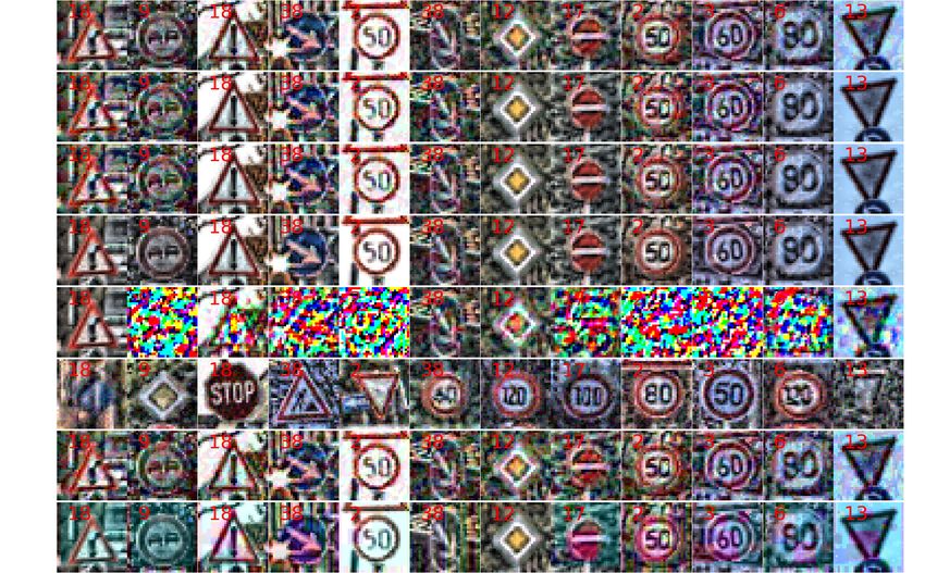
tic image-based classifiers in real-world machine learning                 The concept of white-box attacks and black-box attacks
system applications. More discussions are presented in                  build upon the level of adversary’s knowledge. White-box
Sec 6.                                                                  attacks typically acquire the full knowledge of the model,
                                                                        including model architectures, parameters, loss formula.
2. Background                                                           White-box attack methods generate perturbations based on
                                                                        NN gradients given the detailed knowledge of the model.
2.1. Bayesian neural networks                                           Under Eq. (1), the Fast Gradient Sign Method (FGSM)
    The formulation of Bayesian NN relies on Bayesian                   [13] generates xadv by an one-step update. Basic Itera-
probabilistic modeling with i.i.d. distributions over network           tive Method (BIM) [17] is an iterative version of FGSM
parameters. The Bayesian approach gives a space of param-               with a multi-step update. Projected gradient descent method
eters ω as a distribution p(ω) called the prior, and a likeli-          (PGD) [18] has a similar first-order setup but with ran-
hood distribution p(Y |X, ω), which is a probabilistic model            dom initials. DeepF [20] and Carlini & Wagner’s method
of the model outputs given X and ω. The posterior is pro-               (C&W) [8] have been used to solve Eq. (2).
portional to the likelihood and the prior and the prediction               Black-box attacks have limit/partial knowledge of the
is simply Ep(ω|X,Y ) [p(Y ∗ |X ∗ , ω)]. X ∗ is the test input and       target model. Depending on the portion of the knowledge
Y ∗ is the prediction. However, the inference of the posterior          to the model, it can be further categorized into transfer-
and the prediction are both intractable [4].                            based, score-based, and decision-based black-box attacks.
    Variational Inference (VI) [16], as an approximate prob-            Transfer-based attack uses distillation as a defense strat-
abilistic inference method, is used to resolve this. The ob-            egy by training a substitute model with the knowledge of
jective is to minimize the distance between the approximate             the training data. Momentum Iterative Method (MIM) [11]
variational distribution qθ (ω) for the posterior p(ω|X, Y ).           gives guidance on update direction as an extension of BIM.
The objective is further approximated as the negative Evi-              Score-based black-box attacks only acquire the output prob-
dence Lower                                                             abilities. It estimates the gradients by gradient-free methods
            PnBOund (ELBO). In practice, ELBO is approx-                with limited queries. An example of a score-based attack
imated by i=1 [qω(i) (ω)−log p(ω (i) )−log p(Y |X, ω (i) )],
where ω (i) is the ith Monte Carlo sample from qθ (ω).                  is SPSA [22]. Decision-based black-box attacks solely ac-
ω is reparameterized into (µ, σ) for backpropagation [15,               quire the hard-label predictions. The Square Attack [2] is an
19]. Sampling the network parameters stochastically during              example based on a random search on the decision bound-
training is referred as weight perturbations. The recent ad-            ary.
vancements of weight perturbation method, Flipout, decor-
                                                                        2.3. Input perturbations
relate the gradients within each batch of the data [23], while
boosting the inference process of BNN.                                      Input perturbations to x, as a similar concept to data aug-
                                                                        mentation, are also examined in this paper as they also ex-
2.2. Adversarial Attacks                                                ist in real-world cases. We adopt 6 types of input pertur-
    Adversarial attacks are defined based upon the concept              bation methods to simulate various user cases. Firstly, we
of threat model [6]. Denote f (·) as a classification model,            use the recent advancement Random Erasing (RE) [26]. RE
with original input x and adversarial samples xadv , and y              randomly masks a rectangular region with black color in
denotes the ground-truth label. The adversarial attack is to            x with several masking parameters to determine the size
attack the model f by adding small perturbation on the orig-            of the region. Furthermore, we generate RE with random
inal inputs. This perturbation measured by the Lp norm is               color as masking of the inputs. A typical case is stickers
limited by the perturbation budget ε, that is kx − xadv kp <            on the stop sign and fails a self-driving car. We also adopt
ε. Particularly, we use L∞ in this paper which implies that             the salt-and-pepper noise [3], and speckle noise to simulate
the perturbation to each pixel in x can’t be larger than ε. The         signal interference. This includes the electromagnetic in-
generation of adversarial samples is formulated into two op-            terference (EMI) in unshielded twisted pairs (UTP) in Eth-
timization problems depend on if ε presented. Eq. (1) is to             ernet or adjacent-channel interference in frequency modu-
generate an untargeted adversarial example by maximizing                lation (FM) systems. We use Gaussian/Possion blur on x
the cross-entropy loss function L. The second strategy is               to simulate the system with low data transmission speed,
to find the minimum perturbation as Eq. (2). x0 is one pro-             and/or bandwidth issues.
posed adversarial sample by the generation algorithm.
                                                                        3. Experiments
                     adv                   0
                 x         ← argmax L(x , y)                 (1)        3.1. Evaluated Datasets
                             kx−x0 kp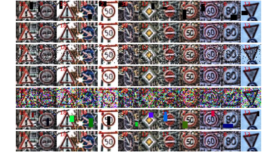
Table 1: Performance Against Input Perturbations. Report Test Accuracy in %.

        Dataset I: GTSRB(German Traffic Sign Recognition Benchmark)
        Methods           Clean        Gaussian      S&P         Poisson             RE           RE Colorful   Speckle
        CNN      Baseline 96.28±0.69 96.19±0.72 76.91±4.37 96.29±0.69                88.76±0.79   72.50±4.52    15.18±2.33
                 Flipout  97.17±0.22 97.19±0.17 84.06±1.00 97.18±0.17                90.45±0.33   82.12±0.55    34.12±3.27
        F-BNN
                 BBB      97.25±0.16 97.27±0.16 80.81±1.61 97.26±0.21                89.81±0.92   79.69±1.99    26.89±2.81
                 Flipout  96.85±0.51 96.87±0.56 75.51±4.49 96.90±0.55                89.93±0.85   72.96±1.60    10.46±4.52
                 BBB      96.93±0.32 96.94±0.35 79.42±1.93 96.93±0.34                88.45±1.32   73.65±2.71    17.48±2.97
        BNN
                 LRT      96.85±0.16 96.83±0.20 75.60±1.13 96.83±0.23                88.64±1.22   71.88±4.22    10.88±2.50
                 VI       95.37±0.41 95.30±0.44 73.33±3.65 95.35±0.40                85.83±1.84   68.91±0.99    10.05±2.42

the training set contains 39, 209 images and 12, 630 in test           between adversarial samples and the original inputs for each
set. The PlansNet has two class labels indicate plane or no-           run. We report the mean L∞ distance between x and xadv
plane given a input image. We use 10% of the data for test-            for different attack methods in the table (e.g. PGD/0.068).
ing. The attack methods discussed in Sec. 2.2 and Sec. 2.3                We also perform training time analysis for BNN and F-
are used in the experiment. The visualization of test images           BNN with various settings in Figure. 1. The model archi-
are shown in Appendix.                                                 tecture, layer setups, and training procedure for different
                                                                       methods are kept identical to address a fair comparison. The
3.2. Evaluation Procedures                                             minimum median time used for training BNN is the Bayes
   Firstly, we train the baseline CNN model, the F-BNN                 By Backprop method, with smaller interquartile range. This
model, and the BNN model. We build all the models fol-                 also holds true for F-BNN training where only BBB and
lowing the VGG-16 architecture, but with stochastic layers             Flipout are used. We observe that BNN requires less com-
in the Bayesian formulation. F-BNN here refers to fully-               puter training time. The same pattern is discovered for both
Bayesian neural network where both feature extractor and               datasets.
classifier are stochastic, while only stochastic classifier pre-
sented in BNN model. Then, we generate different types of
adversarial samples of the test data w.r.t. the baseline CNN
model and test each of the trained model to get the classifi-
cation accuracy against adversarial attacks. Repeating this
procedure for 5 times and averaging the results to get the
mean prediction accuracy and variance. The evaluation pro-
cedure for input perturbations are similar to this procedure.
We report the quantitative results in Table. 1, Table. 2.
                                                                       Figure 1: Training time comparison on GTSRB with
4. Results                                                             stochastic BNN. Left: BNN with only classifier as stochas-
    Table. 1 lists the quantitative results of each model setups       tic. Right: F-BNN with stochasticity on each neural net-
against input perturbations. Results with a clean test input           work layer.
show the CNN baseline is well-trained. Variational Bayes
performs slightly worse. We analysis input perturbations
by groups, a) The Gaussian/Possion noisy blur to the inputs            5. Discussions
won’t affect the model performance. The reason is neu-
                                                                           For adversarial attacks, the PGD achieves best attack
ral network has been proved to have denoising capabilities,
                                                                       performance towards our CNN baseline models with rea-
especially for parameterized distributional noise. b) The F-
                                                                       sonable perturbations. However, BNN and F-BNN also ex-
BNN with the RE/Colorful RE input perturbations has bet-
                                                                       hibit significant robustness gain under PGD attacks. The
ter performance among all cases. c) The S&P/Speckle sig-
                                                                       classification accuracy rises to 80% in F-BNN for GTSRB
nal interference cases has the best attack performance.
                                                                       data. The white-box adversarial samples generated with
    In Table. 2, we report the results of different models
                                                                       Eq. 2 show bipolarity. This indicates the generation algo-
against adversarial attacks on two datasets. For GTSRB
                                                                       rithm needs specific parameter tuning. This is beyond the
dataset, We generate the untargeted adversarial samples us-
                                                                       scope of this work. Bayesian NN also proves to be robust
ing the L∞ threat model with ε = 0.10 and ε = 0.15 on
                                                                       under these cases. The peer comparison between stochastic
both of these two datasets. We perform attacks as previ-
                                                                       setting shows that BNN and F-BNN are analogous, in the
ously discussed in Sec. 2.2. We also evaluate the L∞ norm

                                                                   3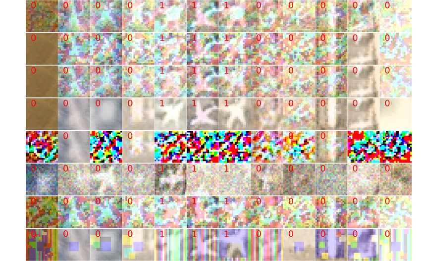
Table 2: Performance Against Adversarial Attacks with different ε and dataset. Report Test Accuracy in %.

    Dataset I: GTSRB(German Traffic Sign Recognition Benchmark)
    L∞ ( = .10)        White-box Attacks                                                      Black-box Attacks
    Methods/Distance    PGD/0.056      FGSM/0.071 BIM/0.049          C&W/0.001   DeepF/0.283   SPSA/0.290 MIM/0.092      Square/0.088
    CNN       Baseline 2.43 ± 0.50 28.79±1.69 28.35±1.65 83.80±6.19              3.97 ± 0.64   3.27 ± 0.12 2.26 ± 0.41   15.26±3.05
              Flipout   77.86±2.57 58.86±1.68 68.08±2.53 95.59±0.27              20.58±1.73    3.75 ± 0.04 61.59±3.00    85.65±4.36
    F-BNN
              BBB       78.78±3.27 59.96±2.01 69.32±2.88 95.76±0.23              20.57±1.90    3.78 ± 0.04 62.86±3.47    80.19±3.37
              Flipout   75.55±2.93 55.71±2.39 65.77±2.42 94.99±0.61              18.57±1.88    3.78 ± 0.06 57.30±2.84    70.54±5.01
              BBB       76.47±1.68 57.13±1.61 66.69±1.58 95.44±0.53              19.47±2.65    3.76 ± 0.05 58.49±2.20    71.65±7.76
    BNN
              LRT       76.78±2.04 57.10±1.86 67.25±1.89 95.55±0.35              19.33±1.42    3.77 ± 0.05 58.90±2.80    76.53±5.79
              VI        73.14±1.89 53.37±1.16 63.51±1.13 93.85±0.59              17.79±2.28    3.75 ± 0.08 53.97±2.18    67.86±8.42
    Dataset I: GTSRB(German Traffic Sign Recognition Benchmark)
    L∞ ( = .15)        White-box Attacks                                                      Black-box Attacks
    Methods/Distance    PGD/0.061      FGSM/0.104 BIM/0.060          C&W/0.002   DeepF/0.285   SPSA/0.293 MIM/0.133      Square/0.132
    CNN       Baseline 2.41 ± 0.51 28.29±1.77 28.32±1.66 79.77±2.49              3.99 ± 0.64   3.20 ± 0.09 2.21 ± 0.39   5.24 ± 1.66
              Flipout   73.28±2.97 42.79±3.68 56.20±4.42 94.94±0.14              20.96±0.84    3.80 ± 0.02 42.86±4.41    73.10±5.62
    F-BNN
              BBB       70.00±2.37 41.91±1.84 53.87±2.13 94.97±0.14              19.92±1.78    3.87 ± 0.04 39.76±1.79    74.51±5.97
              Flipout   69.96±3.26 40.88±0.82 54.65±1.25 94.65±0.49              20.01±0.27    3.75 ± 0.04 37.58±2.41    62.82±4.08
              BBB       70.21±1.75 40.92±1.41 54.23±1.53 94.72±0.38              19.89±1.13    3.83 ± 0.04 38.54±1.89    58.18±9.47
    BNN
              LRT       69.39±2.20 40.48±1.34 53.54±1.44 94.76±0.09              19.11±2.36    3.78 ± 0.07 36.34±1.81    60.43±11.1
              VI        67.35±3.84 39.89±1.89 53.28±2.45 93.23±0.42              18.07±1.75    3.79 ± 0.05 35.12±2.43    53.86±8.77
    Dataset II: PlanesNet(Detect Aircraft in Planet Satellite Image Chips)
    L∞ ( = .10)        White-box Attacks                                                      Black-box Attacks
    Methods/Distance    PGD/0.068      FGSM/0.086 BIM/0.061          C&W/0.005   DeepF/0.349   SPSA/0.212 MIM/0.094      Square/0.080
    CNN       Baseline 1.81 ± 0.37 45.44±2.40 13.50±2.28 68.21±2.13              43.77±4.83    49.65±0.91 1.83 ± 0.36    15.46±1.70
              Flipout   24.51±3.70 57.69±2.37 36.78±4.35 91.13±0.41              54.90±2.84    60.88±0.79 23.14±2.71     75.36±6.81
    F-BNN
              BBB       28.43±5.81 58.51±2.65 40.96±6.94 89.69±0.82              48.54±8.92    66.54±1.06 26.28±5.04     76.20±7.44
              Flipout   23.54±2.67 62.77±1.30 40.31±3.33 91.33±0.76              68.30±1.33    65.58±2.68 24.07±2.25     75.89±2.65
              BBB       22.58±4.24 59.74±4.23 38.69±8.71 91.59±1.35              61.85±5.06    62.94±2.94 22.72±4.20     74.98±4.11
    BNN
              LRT       25.22±1.80 62.59±1.09 42.23±3.93 91.47±1.42              69.33±2.28    65.57±2.16 25.83±2.42     77.79±1.59
              VI        20.72±5.56 55.79±3.38 33.92±6.17 91.19±1.70              65.89±4.76    60.30±2.49 19.91±5.57     72.56±4.02

sense of robustness against white-box adversarial attacks.              6. Conclusion
The results shows inconsistency among different types of
black-box attacks, especially adversarial samples based on                  We highlight several discoveries here. Firstly, the
Eq. 2. For instance, with ε = 0.10, SPSA shows better at-               Bayesian formulation of Neural Network can remarkably
tack performance on GTSRB but MIM has the best attack                   improve the performance of deep learning models, espe-
performance on PlanesNet. SPSA fails every model for GT-                cially when dealing with constrained white-box adversarial
                                                                        attacks. Then, we notice that solely a Bayesian classifier
SRB, still due to the large perturbations to original inputs.
Bayesian NN shows better performance against black-box                  is sufficient to improve model robustness. This decreases
attacks. In some cases, F-BNN has slightly better perfor-               the time and space complexity with fewer parameter dis-
mance compare to BNN but others not. This peer compari-                 tributions. It’s also insignificant when dealing with aug-
son shows similar results with white-box attacks.                       mentation based input perturbations since classical CNN
   Overall, Bayesian NN shows remarkably robustness                     has already shows satisfactory denosing capabilities. Lastly,
                                                                        Bayesian neural network may fail. This happens when deal-
against all types of adversarial attacks except SPSA on
GTSRB. This is due to the large, human-visible pertur-                  ing images with human-visible modifications.
bations generated from SPSA. Larger adversarial pertur-                     In the future, it worth looking at the possible reasons
bations cased by larger ε value makes the model perform                 of good performance on image classification task. For
worse, unless the model has already failed with small per-              instance, benefits of ensemble methods or the feature of
                                                                        Bayesian statistics. Also, it’s interesting to look at the
turbations. BNN achieves comparable performance to F-
BNN in the sense of classification accuracy, for both white-            model robustness against attacks that are developed specif-
box and black-box attacks.                                              ically toward BNNs (e.g. gradient-free adversarial attacks
                                                                        for BNN [24]). The Bayesian posterior observed from BNN
                                                                        can act as the safety precursor of ongoing malicious activi-
                                                                        ties toward the deploy machine learning systems. This leads
                                                                        to the detection of adversarial samples in cybersecurity.

                                                                    4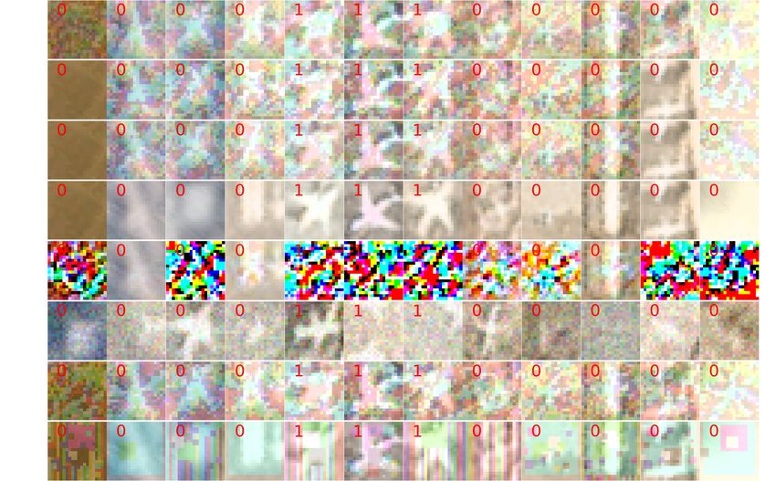
References                                                                [15] Diederik P Kingma, Tim Salimans, and Max Welling. Vari-
                                                                               ational dropout and the local reparameterization trick. arXiv
 [1] Chirag Agarwal, Anh Nguyen, and Dan Schonfeld. Improv-                    preprint arXiv:1506.02557, 2015. 1, 2
     ing robustness to adversarial examples by encouraging dis-
                                                                          [16] Diederik P Kingma and Max Welling. Auto-encoding varia-
     criminative features. In 2019 IEEE International Conference
                                                                               tional bayes. arXiv preprint arXiv:1312.6114, 2013. 1, 2
     on Image Processing (ICIP), pages 3801–3505. IEEE, 2019.
                                                                          [17] Alexey Kurakin, Ian Goodfellow, Samy Bengio, et al. Ad-
     1
                                                                               versarial examples in the physical world, 2016. 2
 [2] Maksym Andriushchenko, Francesco Croce, Nicolas Flam-
                                                                          [18] Aleksander Madry, Aleksandar Makelov, Ludwig Schmidt,
     marion, and Matthias Hein. Square attack: a query-efficient
                                                                               Dimitris Tsipras, and Adrian Vladu. Towards deep learn-
     black-box adversarial attack via random search. In European
                                                                               ing models resistant to adversarial attacks. arXiv preprint
     Conference on Computer Vision, pages 484–501. Springer,
                                                                               arXiv:1706.06083, 2017. 2
     2020. 2
 [3] Jamil Azzeh, Bilal Zahran, and Ziad Alqadi. Salt and pepper          [19] Dmitry Molchanov, Arsenii Ashukha, and Dmitry Vetrov.
     noise: Effects and removal. JOIV: International Journal on                Variational dropout sparsifies deep neural networks. In In-
     Informatics Visualization, 2(4):252–256, 2018. 2                          ternational Conference on Machine Learning, pages 2498–
                                                                               2507. PMLR, 2017. 1, 2
 [4] Charles Blundell, Julien Cornebise, Koray Kavukcuoglu,
     and Daan Wierstra. Weight uncertainty in neural network.             [20] Seyed-Mohsen Moosavi-Dezfooli, Alhussein Fawzi, and
     In International Conference on Machine Learning, pages                    Pascal Frossard. Deepfool: a simple and accurate method to
     1613–1622. PMLR, 2015. 1, 2                                               fool deep neural networks. In Proceedings of the IEEE con-
                                                                               ference on computer vision and pattern recognition, pages
 [5] Luca Cardelli, Marta Kwiatkowska, Luca Laurenti, Nicola
                                                                               2574–2582, 2016. 2
     Paoletti, Andrea Patane, and Matthew Wicker. Statistical
     guarantees for the robustness of bayesian neural networks.           [21] Yuchi Tian, Kexin Pei, Suman Jana, and Baishakhi Ray.
     arXiv preprint arXiv:1903.01980, 2019. 1                                  Deeptest: Automated testing of deep-neural-network-driven
 [6] Nicholas Carlini, Anish Athalye, Nicolas Papernot, Wieland                autonomous cars. In Proceedings of the 40th international
     Brendel, Jonas Rauber, Dimitris Tsipras, Ian Goodfellow,                  conference on software engineering, pages 303–314, 2018.
     Aleksander Madry, and Alexey Kurakin. On evaluating                       1
     adversarial robustness. arXiv preprint arXiv:1902.06705,             [22] Jonathan Uesato, Brendan O’donoghue, Pushmeet Kohli,
     2019. 2                                                                   and Aaron Oord. Adversarial risk and the dangers of evalu-
 [7] Nicholas Carlini and David Wagner. Adversarial examples                   ating against weak attacks. In International Conference on
     are not easily detected: Bypassing ten detection methods. In              Machine Learning, pages 5025–5034. PMLR, 2018. 2
     Proceedings of the 10th ACM Workshop on Artificial Intelli-          [23] Yeming Wen, Paul Vicol, Jimmy Ba, Dustin Tran, and
     gence and Security, pages 3–14, 2017. 1                                   Roger Grosse.       Flipout: Efficient pseudo-independent
 [8] Nicholas Carlini and David Wagner. Towards evaluating the                 weight perturbations on mini-batches.         arXiv preprint
     robustness of neural networks. In 2017 ieee symposium on                  arXiv:1803.04386, 2018. 1, 2
     security and privacy (sp), pages 39–57. IEEE, 2017. 1, 2             [24] Matthew Yuan, Matthew Wicker, and Luca Laurenti.
 [9] Planet’s Open California dataset. Planes in satellite imagery,            Gradient-free adversarial attacks for bayesian neural net-
     2018. 1, 2                                                                works. arXiv preprint arXiv:2012.12640, 2020. 4
[10] Yinpeng Dong, Qi-An Fu, Xiao Yang, Tianyu Pang, Hang                 [25] Huan Zhang, Hongge Chen, Zhao Song, Duane Boning, In-
     Su, Zihao Xiao, and Jun Zhu. Benchmarking adversar-                       derjit S Dhillon, and Cho-Jui Hsieh. The limitations of ad-
     ial robustness on image classification. In Proceedings of                 versarial training and the blind-spot attack. arXiv preprint
     the IEEE/CVF Conference on Computer Vision and Pattern                    arXiv:1901.04684, 2019. 1
     Recognition, pages 321–331, 2020. 1                                  [26] Zhun Zhong, Liang Zheng, Guoliang Kang, Shaozi Li, and
[11] Yinpeng Dong, Fangzhou Liao, Tianyu Pang, Hang Su, Jun                    Yi Yang. Random erasing data augmentation. In Proceedings
     Zhu, Xiaolin Hu, and Jianguo Li. Boosting adversarial at-                 of the AAAI Conference on Artificial Intelligence (AAAI),
     tacks with momentum. In Proceedings of the IEEE con-                      2020. 2
     ference on computer vision and pattern recognition, pages
     9185–9193, 2018. 2
[12] Yinpeng Dong, Hang Su, Jun Zhu, and Fan Bao. Towards
     interpretable deep neural networks by leveraging adversarial
     examples. arXiv preprint arXiv:1708.05493, 2017. 1
[13] Ian J Goodfellow, Jonathon Shlens, and Christian Szegedy.
     Explaining and harnessing adversarial examples. arXiv
     preprint arXiv:1412.6572, 2014. 1, 2
[14] Sebastian Houben, Johannes Stallkamp, Jan Salmen, Marc
     Schlipsing, and Christian Igel. Detection of traffic signs
     in real-world images: The German Traffic Sign Detection
     Benchmark. In International Joint Conference on Neural
     Networks, number 1288, 2013. 1, 2

                                                                      5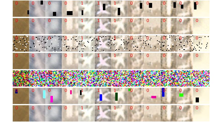
A. Appendix
A.1. Evaluation Results on PlanesNet Dataset
We list the classification results of PlanesNet Dataset in Table. 3 and Table. 4. The PlanesNet Dataset is open-source
online. The objective is to classify the existence of aircrafts in surveillance satellite images. The PlanesNet has two class
labels indicate plane or not plane. PlanesNet is another good example to demonstrate the potential benefits to the engineering
applications in a safety-critical domain. Table. 3 is the results against input perturbations. Table. 4 is the results against
adversarial attacks.
Table 3: Performance Against Input Perturbations. Report Test Accuracy in %.
Dataset II: PlanesNet(Detect Aircraft in Planet Satellite Image Chips)
Methods Clean Gaussian S&P Poisson RE RE Colorful Speckle
CNN Baseline 98.19±0.37 98.21±0.31 86.76±1.29 98.22±0.38 93.16±0.60 88.99±0.80 74.76±0.41
Flipout 97.83±0.12 97.79±0.21 91.91±0.41 97.86±0.15 93.06±0.24 89.43±0.75 74.80±0.90
F-BNN
BBB 96.50±0.69 96.59±0.55 87.85±1.84 96.59±0.70 91.14±0.92 88.39±0.91 75.33±0.91
Flipout 98.55±0.28 98.44±0.28 84.06±3.02 98.53±0.26 92.21±0.57 89.44±0.52 74.79±0.23
BBB 98.73±0.23 98.65±0.27 83.84±2.96 98.71±0.25 91.63±0.70 88.98±0.67 75.04±0.32
BNN
LRT 98.88±0.12 98.87±0.11 83.00±1.88 98.89±0.11 92.30±0.55 89.04±0.21 74.78±0.12
VI 96.41±2.72 96.23±2.82 82.73±3.41 96.34±2.67 89.86±2.31 87.01±1.33 72.96±3.25
Table 4: Performance Against Adversarial Attacks. Report Test Accuracy in %.
Dataset II: PlanesNet(Detect Aircraft in Planet Satellite Image Chips)
L∞ ( = .10) White-box Attacks Black-box Attacks
Methods/Distance PGD/0.068 FGSM/0.086 BIM/0.061 C&W/0.005 DeepF/0.349 SPSA/0.212 MIM/0.094 Square/0.080
CNN Baseline 1.81 ± 0.37 45.44±2.40 13.50±2.28 68.21±2.13 43.77±4.83 49.65±0.91 1.83 ± 0.36 15.46±1.70
Flipout 24.51±3.70 57.69±2.37 36.78±4.35 91.13±0.41 54.90±2.84 60.88±0.79 23.14±2.71 75.36±6.81
F-BNN
BBB 28.43±5.81 58.51±2.65 40.96±6.94 89.69±0.82 48.54±8.92 66.54±1.06 26.28±5.04 76.20±7.44
Flipout 23.54±2.67 62.77±1.30 40.31±3.33 91.33±0.76 68.30±1.33 65.58±2.68 24.07±2.25 75.89±2.65
BBB 22.58±4.24 59.74±4.23 38.69±8.71 91.59±1.35 61.85±5.06 62.94±2.94 22.72±4.20 74.98±4.11
BNN
LRT 25.22±1.80 62.59±1.09 42.23±3.93 91.47±1.42 69.33±2.28 65.57±2.16 25.83±2.42 77.79±1.59
VI 20.72±5.56 55.79±3.38 33.92±6.17 91.19±1.70 65.89±4.76 60.30±2.49 19.91±5.57 72.56±4.02
Dataset II: PlanesNet(Detect Aircraft in Planet Satellite Image Chips)
L∞ ( = .15) White-box Attacks Black-box Attacks
Methods/Distance PGD/0.085 FGSM/0.127 BIM/0.084 C&W/0.007 DeepF/0.352 SPSA/0.217 MIM/0.139 Square/0.113
CNN Baseline 1.81 ± 0.37 50.96±2.07 12.79±2.37 63.92±1.99 45.14±4.89 49.03±0.67 1.81 ± 0.36 12.53±2.90
Flipout 16.71±2.83 56.17±1.66 20.74±2.99 89.33±0.86 52.86±4.97 61.99±0.60 17.28±3.62 64.91±7.99
F-BNN
BBB 21.33±5.90 57.48±0.57 23.98±3.64 87.85±1.27 52.00±3.38 68.57±1.92 19.77±4.45 68.76±7.46
Flipout 19.33±4.21 63.91±4.22 25.28±5.88 90.16±0.56 67.64±3.04 67.35±2.32 22.76±5.80 72.38±1.57
BBB 16.85±3.95 63.92±3.16 24.04±3.61 90.32±0.84 65.43±2.05 67.89±2.97 19.54±4.39 72.58±2.80
BNN
LRT 19.01±4.72 63.54±2.56 24.27±4.83 90.85±0.34 69.08±1.94 67.09±1.24 21.52±5.07 70.67±2.45
VI 24.82±7.63 65.39±4.98 32.04±9.46 88.21±3.27 68.59±3.37 67.99±4.05 30.16±10.1 72.96±1.64
A.2. Visualization of the Data
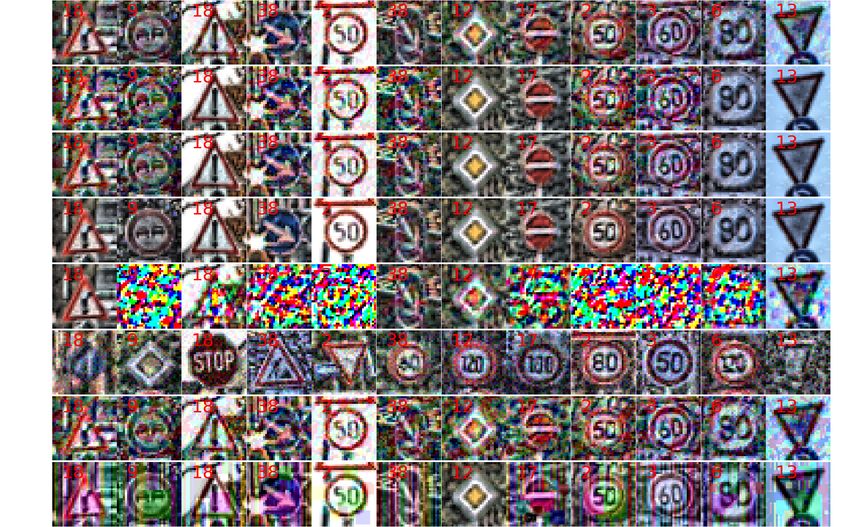
We visualize the data with input perturbations in Fig. 2. The first 12 samples in the test dataset are chosen with their
correct class labels indicated at the top-left corner. The types of input perturbation are Random Erasing, Gaussian, Salt-and-
Pepper, Possion, Speckle, Random Erasing Colorful, Clean. Similarly, the adversarial test samples are visualized in Fig. 3,
with different perturbation budgets ε = 0.10 for (a) & (b), ε = 0.15 for (c) & (d).
6(a) PlanesNet with Input Perturbations (b) GTSRB with Input Perturbations
Figure 2: Visualization of applying input perturbations to PlanesNet and GTSRB. From top to bottom, the methods are: RE,
Gaussian, S&P, Possion, Speckle, RE Colorful, Clean. The ground-truth for class labels are indicated at the top-left corner
of each data plot. (a) PlanesNet. (b) GTSRB
(a) Adversarial Samples for PlanesNet: ε = 0.10 (b) Adversarial Samples for GTSRB: ε = 0.10
(c) Adversarial Samples for PlanesNet: ε = 0.15 (d) Adversarial Samples for GTSRB: ε = 0.15
Figure 3: Visualization of applying input perturbations to PlanesNet and GTSRB. From top to bottom, the methods are:
PGD, FGSM, BIM, C&W, DeepF, SPSA, MIM, Square. The ground-truth for class labels are indicated at the top-left corner
of each data plot. (a) PlanesNet. (b) GTSRB
7A.3. Training Time Analysis
The training time of different methods on both two datasets are compared in Fig. 4 and Fig. 5. We can see BNNs require
less training time.
(a) BNN Training time on GTSRB dataset (b) F-BNN Training time on GTSRB dataset
Figure 4: Training time comparison with stochastic BNN. The figures for PlaneNet are reported in Fig. 5. (a) BNN with only
classifier as stochastic. (b) F-BNN with stochasticity on every neural network layers.
(a) BNN on PlanesNet (b) F-BNN on PlanesNet
Figure 5: Training time comparison with stochastic BNN. (a) BNN with only classifier as stochastic. (b) F-BNN with
stochasticity on every neural network layers.
8You can also read