LOCAL CRITIC TRAINING OF DEEP NEURAL NET-WORKS - OpenReview
←
→
Page content transcription
If your browser does not render page correctly, please read the page content below

Under review as a conference paper at ICLR 2019

L OCAL C RITIC T RAINING                             OF    D EEP N EURAL N ET-
WORKS

 Anonymous authors
 Paper under double-blind review

                                           A BSTRACT

         This paper proposes a novel approach to train deep neural networks by unlocking
         the layer-wise dependency of backpropagation training. The approach employs
         additional modules called local critic networks besides the main network model to
         be trained, which are used to obtain error gradients without complete feedforward
         and backward propagation processes. We propose a cascaded learning strategy for
         these local networks. In addition, the approach is also useful from multi-model
         perspectives, including structural optimization of neural networks, computation-
         ally efficient progressive inference, and ensemble classification for performance
         improvement. Experimental results show the effectiveness of the proposed ap-
         proach and suggest guidelines for determining appropriate algorithm parameters.

1   I NTRODUCTION
In recent days, deep learning has been remarkably advanced and successfully applied in numerous
fields (LeCun et al., 2015). A key mechanism behind the success of deep neural networks is that
they are capable of extracting useful information progressively through their layered structures. It
is an increasing trend that more and more complex deep neural network structures are developed
in order to solve challenging real-world problems, e.g., He et al. (2016b). Training of deep neural
networks is based on backpropagation in most cases, which basically works in a sequential and
synchronous manner. During the feedforward pass, the input data is processed through the hidden
layers to produce the network output; during the feedback pass, the error gradient is propagated
back through the layers to update each layer’s weight parameters. Therefore, training of each layer
has dependency on all the other layers, which causes the issue of locking (Jaderberg et al., 2017).
This is undesirable in some cases, e.g., a system consisting of several interacting models, a model
distributed across multiple computing nodes, etc.
There have been attempts to remove the locking constraint. In Carreira-Perpinan & Wang (2014),
the method of auxiliary coordinates (MAC) is proposed. It replaces the original loss minimization
problem with an equality-constrained optimization problem by introducing an auxiliary variable
for each data and each hidden unit. Then, solving the problem is formulated as iteratively solving
several sub-problems independently. A similar approach using the alternating direction method of
multipliers (ADMM) is proposed in Taylor et al. (2016). It also employs an equality-constrained
optimization but with different auxiliary variables, so that resulting sub-problems have closed form
solutions. However, these methods are not scalable to deep learning architectures such as convolu-
tional neural networks (CNNs).
The method proposed in Jaderberg et al. (2017), called decoupled neural interface (DNI), directly
synthesizes estimated error gradients, called synthetic gradients, using an additional small neural
network for training a layer’s weight parameters. As long as the synthetic gradients are close to
the actual backpropagated gradients, each layer does not need to wait until the error at the output
layer is backpropagated through the preceding layers, which allows independent training of each
layer. However, this method suffers from performance degradation when compared to regular back-
propagation (Czarnecki et al., 2017a). The idea of having additional modules supporting the layers
of the main model is also adopted in Czarnecki et al. (2017a), where the additional modules are
trained to approximate the main model’s outputs instead of error gradients. Due to this, however,
the method does not resolve the issue of update locking, and in fact, the work does not intend to
design a non-sequential learning algorithm.

                                                 1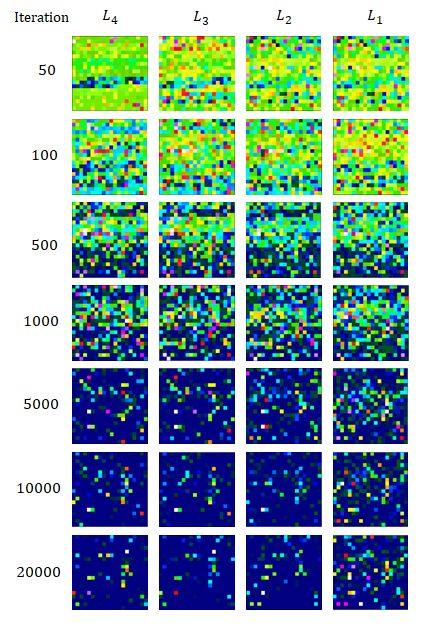
Under review as a conference paper at ICLR 2019

Figure 1: Learning processes of DNI (Jaderberg et al., 2017) and the proposed local critic training.
The black, green, and blue arrows indicate feedforward passes, an error gradient flow, and loss
comparison, respectively.

In this paper, we propose a novel approach for non-sequential learning, called local critic training.
The key idea is that additional modules besides the main neural network model are employed, which
we call local critics, in order to indirectly deliver error gradients to the main model for training with-
out backpropagation. In other words, a local critic located at a certain layer group is trained in such
a way that the derivative of its output serves as the error gradient for training of the corresponding
layers’ weight parameters. Thus, the error gradient does not need to be backpropagated, and the
feedforward operations and gradient-descent learning can be performed independently. Through
extensive experiments, we examine the influences of the network structure, update frequency, and
total number of local critics, which provide not only insight into operation characteristics but also
guidelines for performance optimization of the proposed method.
In addition to the capability of implementing training without locking, the proposed approach can be
exploited for additional important applications. First, we show that applying the proposed method
automatically performs structural optimization of neural networks for a given problem, which has
been a challenging issue in the machine learning field. Second, a progressive inference algorithm
using the network trained with the proposed method is presented, which can adaptively reduce the
computational complexity during the inference process (i.e., test phase) depending on the given data.
Third, the network trained by the proposed method naturally enables ensemble inference that can
improve the classification performance.

2     P ROPOSED A PPROACH
2.1   L OCAL C RITIC T RAINING

The basic idea of the proposed approach is to introduce additional local networks, which we call
local critics, besides the main network model, so that they eventually provide estimates of the output
of the main network. Each local critic network can serve a group of layers of the main model by
being attached to the last layer of the group. The proposed architecture is illustrated in Figure 1,
where fi is the ith layer group (containing one or more layers), hi is the output of fi , and hN is the
final output of the main model having N layer groups:
                                              hi = fi (hi−1 )                                       (1)
ci is the local critic network for fi , which is expected to approximate hN based on hi , i.e.,
                                               ci (hi ) ≈ hN                                        (2)
Then, this can be used to approximate the loss function of the main network, LN = l(hN , y), which
is used to train fi , by
                                             Li = l(ci (hi ), y)                                    (3)

                                                    2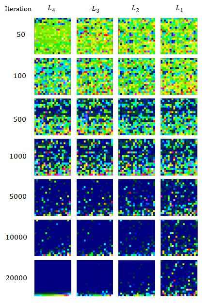
Under review as a conference paper at ICLR 2019

for i = 1, ..., N − 1, i.e.,
                                              Li ≈ LN                                              (4)
where y is the training target and l is the loss function such as cross-entropy or mean-squared error.
Then, the error gradient for training fi is obtained by differentiating Li with respect to hi , i.e.,
                                                      ∂Li
                                              δi =                                                 (5)
                                                      ∂hi
which can be used to train the weight parameters of fi , denoted by θi , via a gradient-descent rule:
                                                            ∂hi
                                         θi ← θi − η δi                                            (6)
                                                            ∂θi
where η is a learning rate. Note that the final layer group hN does not require a local critic network
and can be trained using the regular backproagation because the final output of the main network is
directly available. Therefore, the update of fi does not need to wait until its output hi propagates
till the end of the main network and the error gradient is backpropagated; it can be performed when
the operations from (2) to (5) are done. For ci , we usually use a simple model so that the operations
through ci are simpler than those through fi+1 till fN .
While the dependency of fi on fj (j > i) during training is resolved in this way, there still exists
the dependency of ci on fj (j > i), because training ci requires its ideal target, i.e., hN , which is
available from fN only after the feedforward pass is complete. In order to resolve this problem, we
use an indirect, cascaded approach, where ci is trained so that its training loss targets the training
loss for ci+1 1 :
                                        Lci = l(Li , Li+1 )                                        (7)
In other words, training of ci can be performed once the loss for ci+1 is available.
Figure 1 compares the proposed architecture with the existing DNI approach that also employs local
networks besides the main network to resolve the issue of locking (Jaderberg et al., 2017). In DNI,
the local network ci directly estimates the error gradient, i.e.,
                                                        ∂LN
                                           ci (hi ) ≈                                              (8)
                                                        ∂hi
so that each layer group of the main model can be updated without waiting for the forward and back-
ward propagations in the subsequent layers. And, to update ci , the error gradient for fi+1 estimated
by ci+1 is backpropagated through fi+1 and is used as the (estimated) target for ci . Therefore,
all the necessary computations in the forward and backward passes can be locally confined. The
performance of the two methods will be compared in Section 3.

2.2   S TRUCTURAL OPTIMIZATION

In many cases, determining an appropriate structure of neural networks for a given problem is not
straightforward. This is usually done through trial-and-error, which is extremely time-consuming.
There have been studies to automate the structural optimization process (Cortes et al., 2017; Feng &
Darrell, 2015; Kwok & Yeung, 1997; Reed, 1993), but this issue still remains very challenging.
In deep learning, the problem of structural optimization is even more critical. Large-sized networks
may easily show overfitting. Even if large networks may produce high accuracy, they take signif-
icantly large amounts of memory and computation, which is undesirable especially for resource-
constrained cases such as embedded and mobile systems. Therefore, it is highly desirable to find an
optimal network structure that is sufficiently small while the performance is kept reasonably good.
During local critic training, each local critic network is trained to estimate the output of the main
network eventually. Therefore, once the training of the proposed architecture finishes, we obtain
different networks that are supposed to have similar input-output mappings but have different struc-
tures and possibly different accuracy, i.e., multiple sub-models and one main model (see Figure 2b).
Here, a sub-model is composed of the layers on the path from the input to a certain hidden layer
    1
      We found that this is more effective than directly forcing ci to approximate ci+1 using Lci =
l(ci (hi ), ci+1 (hi+1 )).

                                                  3
Under review as a conference paper at ICLR 2019

Algorithm 1: Progressive inference
    Input: data x, threshold t
    Model: sub-model ci , main-model f
    Initialize: classif ication = 0.
    for i = 1 to N − 1 do
        if max softmax(ci (x)) > t then
           classif ication = argmax softmax(ci (x))
           break
        end if
    end for
    if classif ication == 0 then
        # if all sub-models are not confident
        classif ication = argmax softmax(f (x))
    end if

and its local critic network. Among the sub-models, we can choose one as a structure-optimized
network by considering the trade-off relationship between the complexity and performance.
It is worth mentioning that our structural optimization approach can be performed instantly after
training of the model, whereas many existing methods for structural optimization require iterative
search processes, e.g., Zoph & Le (2017).

2.3    P ROGRESSIVE INFERENCE

We propose another simple but effective way to utilize the sub-models obtained by the proposed
approach for computational efficiency, which we call progressive inference. Although small sub-
models (e.g., sub-model 1) tend to show low accuracy, they would still perform well for some data.
For such data, we do not need to perform the full feedforward pass but can take the classification
decision by the sub-models. Thus, the basic idea of the progressive inference is to finish infer-
ence (i.e., classification) with a small sub-model if its confidence on the classification result is high
enough, instead of completing the full feedforward pass with the main model, which can reduce the
computational complexity. Here, the softmax outputs for all classes are compared and the maximum
probability is used as the confidence level. If it is higher than a threshold, we take the decision by the
sub-model; otherwise, the feedforward pass continues. The proposed progressive inference method
is summarized in Algorithm 12 .

2.4    E NSEMBLE INFERENCE

In recent deep learning systems, it is popular to use ensemble approaches to improve performance
in comparison to single models, where multiple networks are combined for producing final results,
e.g., He et al. (2016a); Szegedy et al. (2015). The sub-models and main model obtained by applying
the proposed local critic training approach can be used for ensemble inference. Figure 4a depicts
how the sub-models and the main model can work together to form an ensemble classifier. We take
the simplest way to combine them, i.e., summation of the networks’ outputs.

3     E XPERIMENTS

We conduct extensive experiments to examine the performance of the proposed method in various
aspects. We use the CIFAR-10 and CIFAR-100 datasets (Krizhevsky, 2009) with data augmentation.
We employ a VGG-like CNN architecture with batch normalization and ReLU activation functions,
which is shown in Figure 2a. Note that this structure is the same to that used in Czarnecki et al.
(2017a). It has three local critic networks, thus four layer groups that can be trained independently
are formed (i.e., N =4). The local critic networks are also CNNs, and their structures are kept as
    2
      Our method shares some similarity with the anytime prediction scheme (Larsson et al., 2017; Huang et al.,
2018) that produces outputs according to the given computational budget. However, ours does not require
particular network structures (such as multi-scale dense network (Huang et al., 2018) or FractalNet (Larsson
et al., 2017)) but works with generic CNNs.

                                                      4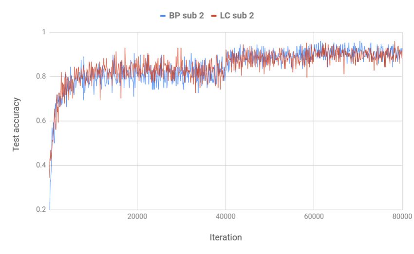
Under review as a conference paper at ICLR 2019

                        (a)                                                 (b)

Figure 2: (a) Network structure of the proposed approach using three local networks for CIFAR-10.
LC1, LC2, and LC3 are local critic networks, each of which contains one convolutional layer. For
CIFAR-100, the final fc10 layers of the main network and the local critic networks are replaced with
fc100. (b) Sub-models and main model obtained by the proposed approach.

                   (a) CIFAR-10                                       (b) CIFAR-100

Figure 3: Training loss values of the main model and each sub-model with respect to the training
iteration.

simple as possible in order to minimize the computational complexity for computing the estimated
error gradient given by (5).
We use the stochastic gradient descent with a momentum of 0.9 for the main network and the Adam
optimization with a fixed learning rate of 10−4 for the local networks. The L2 regularization is
used with 5 × 10⁻⁴ for the main network. For the loss functions in (3) and (7), the cross-entropy
and the L1 loss are used, respectively, which is determined empirically. The batch size is set to
128, and the maximum training iteration is set to 80,000. The learning rate for the main network
is initialized to 0.1 and dropped by an order of magnitude after 40,000 and 60,000 iterations. The
Xavier method is used for initialization of the network parameters. All experiments are performed
using TensorFlow. We conduct all the experiments five times with different random seeds and report
the average accuracy.

3.1   P ERFORMANCE EVALUATION

Figure 3 shows how the loss values of the main network and each local critic network, i.e., Li in
(3), evolve with respect to the training iteration. The graphs show that the local critic networks suc-
cessfully learn to approximate the main network’s loss with high accuracy during the whole training
process. The local critic network farthest from the output side (i.e., L1 ) shows larger loss values
than the others, which is due to the inaccuracy accumulated through the cascaded approximation.
The classification performance of the proposed local critic training approach is evaluated in Table
1. For comparison, the performance of the regular backpropagation, DNI (Jaderberg et al., 2017),
and critic training (Czarnecki et al., 2017a) is also evaluated. Although the critic training method
is not for removing update locking, we include its result because it shares some similarity with our
approach, i.e., additional modules to estimate the main network’s output. In all three methods, each
additional module is composed of a convolutional layer and an output layer. In the case of the
proposed method, we test different numbers of local critic networks. Figure 2a shows the structure

                                                  5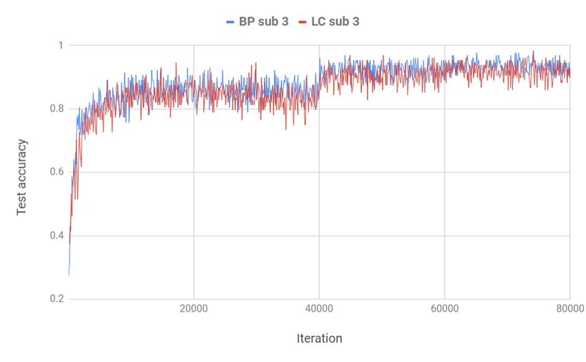
Under review as a conference paper at ICLR 2019

Table 1: Average test accuracy (%) of backpropagation (BP), DNI (Jaderberg et al., 2017), critic
training (Czarnecki et al., 2017a), and proposed local critic training (LC). The numbers of local
networks used are shown in the parentheses. The standard deviation values are also shown.

      Dataset               BP            DNI (3)          Critic (3)            LC (1)          LC (3)          LC (5)
      CIFAR-10         93.93 ±0.20       64.86 ±0.42      91.92 ±0.30        92.06 ±0.20       92.39 ±0.09      91.38 ±0.20
      CIFAR-100        75.14 ±0.18       36.53 ±0.64      69.07 ±0.25        73.61 ±0.31       69.91 ±0.50      63.53 ±0.24

Table 2: Average test accuracy (%) with respect to the number of layers in the local critic networks.
[a, b, c] means that the numbers of convolutional layers in LC1, LC2, and LC3 are a, b, and c,
respectively.

      Dataset     [1,1,1] (default)     [3,3,3]        [5,5,5]         [3,2,1]       [1,2,3]        [5,4,3]          [3,4,5]
      CIFAR-10      92.39 ±0.09       92.36 ±0.22   91.72 ±0.19      92.07 ±0.21   92.20 ±0.12    92.10 ±0.16    91.90 ±0.16
      CIFAR-100     69.91 ±0.50       70.02 ±0.29   70.34 ±0.16      70.06 ±0.64   69.81 ±0.33    70.87 ±0.40    69.93 ±0.56

with three local critic networks. When only one local network is used, it is located at the place of
LC2 in Figure 2a. When five local networks are used, they are placed after every two layers of the
main network.
When compared to the result of backpropagation, the proposed approach successfully decouples
training of the layer groups at a small expense of accuracy decrease (note that the performance of
the proposed method can be made closer to that of backpropagation using different structures, as
will be shown in Tables 2 and Figure 4b). The degradation of the accuracy and standard deviation
of our method is larger for CIFAR-100, which implies that the influence of gradient estimation is
larger for more complex problems. When more local critic networks are used, the accuracy tends
to decrease more due to higher reliance on predicted gradients rather than true gradients, while
more layer groups can be trained independently. Thus, there exists a trade-off between the accuracy
and unlocking effect. The DNI method shows poor performance as in (Czarnecki et al., 2017a).
The proposed method shows performance improvement by 0.4% and 0.9% over the critic training
method, both with three local networks, for the two datasets, respectively, which are found to be
statistically significant using Mann-Whitney tests at a significance level of 0.05. This shows the
efficacy of the cascaded learning scheme of the local networks in our method.

3.2     S TRUCTURES OF LOCAL CRITIC NETWORKS

We examine the influence of the structures of the local critic networks in our method. Two aspects
are considered, one about the influence of the overall complexity of the local networks and the other
about the relative complexities of the local networks for good performance. For this, we change
the number of convolutional layers in each local critic network, while keeping the other structural
parameters unchanged.
The results for various structure combinations of the three local critic networks are shown in Table
2. As the number of convolutional layers increase for all local networks (the first three cases in
the table), the accuracy for CIFAR-100 slightly increases from 69.91% (with one convolutional
layer) to 70.02% (three convolutional layers) and 70.34% (five convolutional layers), whereas for
CIFAR-10 the accuracy slightly decreases when five convolutional layers are used. A more complex
local network can learn better the target input-output relationship, which leads to the performance
improvement for CIFAR-100. For CIFAR-10, on the other hand, the network structure with five
convolutional layers seems too complex compared to the data to learn, which causes the performance
drop.
Next, the numbers of layers of the local networks are adjusted differently in order to investigate
which local networks should be more complex for good performance. The results are shown in
the last four columns of Table 2. Overall, it is more desirable to use more complex structures for
the local networks closer to the input side of the main model. For instance, LC1 and LC3 are
supposed to learn the relationship from h1 to h4 and that from h3 to h4 , respectively. More layers

                                                                 6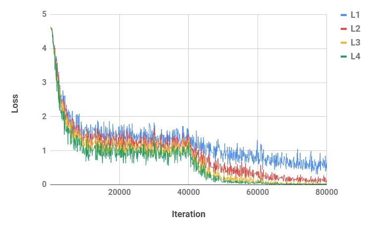
Under review as a conference paper at ICLR 2019

 Table 3: Average test accuracy (%) with respect to the update frequency of local critic networks.

            Dataset          1/1           1/2               1/3           1/4           1/5
            CIFAR-10         92.39 ±0.09   91.91 ±0.19       91.78 ±0.18   91.57 ±0.12   91.35 ±0.17
            CIFAR-100        69.91 ±0.50   67.99 ±0.49       67.76±0.19    66.74 ±0.41   66.39 ±0.39

Table 4: Average test accuracy (%) of the sub-models produced by local critic training and the
networks trained by regular backpropagation.

      Dataset         BP sub 1      LC sub 1      BP sub 2          LC sub 2      BP sub 3      LC sub 3
      CIFAR-10        74.46 ±0.91   85.24 ±0.49   88.03 ±0.87       90.53 ±0.15   92.05 ±0.24   92.29 ±0.09
      CIFAR-100       47.58 ±1.10   55.39 ±0.57   61.79 ±0.92       63.62 ±0.31   67.81 ±0.22   67.54 ±0.70

are involved from h1 to h4 in the main network, so the mapping that LC1 should learn would be
more complicated, requiring a network structure with sufficient modeling capability.

3.3     P ERIODIC UPDATE OF LOCAL CRITIC NETWORKS

A way to increase the efficiency of the proposed approach is to update the local critic networks not at
every iteration but only periodically. This may degrade the accuracy but has two benefits. First, the
amount of computation required to update the local networks can be reduced. Second, the burden
of the communication between the layer groups also can be reduced. These benefits will be more
significant when the local networks have larger sizes.
For the default structure shown in Figure 2a, we compare different update frequency in Table 3. It
is noticed that the accuracy only slightly decreases as the frequency decreases. When the update
frequency is a half of that for the main network (i.e., 1/2), the accuracy drops by 0.48% and 1.92%
for the two datasets, respectively. Then, the decrease of the accuracy is only 0.56% for CIFAR-10
and 1.60% for CIFAR-100 when the update frequency decreases from 1/2 to 1/5.

3.4     S TRUCTURAL OPTIMIZATION

Table 4 compares the performance of the sub-models, and Table 5 shows the complexities of the
sub-models in terms of the amount of computation for a feedforward pass and the number of weight
parameters. A larger network (e.g., sub-model 3) shows better performance than a smaller network
(e.g., sub-model 1), which is reasonable due to the difference in learning capability with respect to
the model size. The largest sub-model (sub-model 3) shows similar accuracy to the main model
(92.29% vs. 92.39% for CIFAR-10 and 67.54% vs. 69.91% for CIFAR-100), while the complex-
ity is significantly reduced. For CIFAR-10, the computational complexity in terms of the number
of floating-point operations (FLOPs) and the memory complexity are reduced to only about 30%
(15.72 to 4.52 million FLOPs, and 7.87 to 2.26 million parameters), as shown in Table 5. If an
absolute accuracy reduction of 1.86% (from 92.39% to 90.53%) is allowed by taking sub-model 2,
the reduction of complexity is even more remarkable, up to about one ninth.
In addition, the table also shows the accuracy of the networks that have the same structures with the
sub-models but are trained using regular backpropagation. Surprisingly, such networks do not easily
reach accuracy comparable to that of the sub-models obtained by local critic training, particularly
for smaller networks (e.g., 74.46% vs. 85.24% with sub-model 1 for CIFAR-10). We think that
joint training of the sub-models in local critic training helps them to find better solutions than those
reached by independent regular backpropagation.
Therefore, these results demonstrate that a structurally optimized network can be obtained at a cost
of a small loss in accuracy by local critic training, which may not be attainable by trial-and-error
with backpropagation.

                                                         7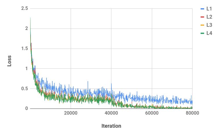
Under review as a conference paper at ICLR 2019

Table 5: FLOPs required for a feedforward pass and numbers of model parameters in the sub-models
and main model for CIFAR-10. Note that sub-model 2 has less FLOPs and parameters than sub-
model 1 due to the pooling operation in sub-model 2.

                            model             FLOP          # of parameters
                            Sub-model 1       2.85M                1.42M
                            Sub-model 2       1.76M                0.88M
                            Sub-model 3       4.52M                2.26M
                            Main model       15.72M                7.87M

Table 6: Average FLOPs and accuracy of progressive inference for test data of CIFAR-10 when the
threshold is set to 0.9 or 0.95.

                                                          FLOP       Accuracy (%)
                       Progressive inference (0.9)        2.90M       91.18 ±0.10
                       Progressive inference (0.95)       3.05M       91.75 ±0.16
                       Main model                         15.72M      92.39 ±0.09

3.5   P ROGRESSIVE INFERENCE

We apply the progressive inference algorithm shown in Algorithm 1 to the trained default network
for CIFAR-10 with the threshold set to 0.9 or 0.95. The results are shown in Table 6. The feedfor-
ward pass ends at different sub-models for different test data, and the average FLOPs over all test
data are shown. When the threshold is 0.9, with only a slight loss of accuracy (92.39% to 91.18%),
the computational complexity is reduced significantly, which is only 18.45% of that of the main
model. When the threshold increases to 0.95, the accuracy loss becomes smaller (only 0.64%),
while the complexity reduction remains almost the same (19.40% of the main model’s complexity).

3.6   E NSEMBLE INFERENCE

The results of ensemble inference using the sub-models and main model are shown in Figure 4b.
Using an ensemble of the three sub-models, we observe improved classification accuracy (92.68%
and 70.86% for the two datasets, respectively) in comparison to the main model. The performance
is further enhanced by an ensemble of both the three sub-models and the main model (92.79%
and 71.86%). The improvement comes from the complementarity among the models, particularly
between the models sharing a smaller number of layers. For instance, we found that sub-model 3
and the main model tend to show coincident classification results for a large portion of test data, so
their complementarity is not significant; on the other hand, more data are classified differently by
sub-model 1 and the main model, where we mainly observe performance improvement. Instead of
the simple summation, there could be a better method to combine the models, which is left for future
work.

4     C ONCLUSION

In this paper, we proposed the local critic training approach for removing the inter-layer locking
constraint in training of deep neural networks. In addition, we proposed three applications of the
local critic training method: structural optimization of neural networks, progressive inference, and
ensemble classification. It was demonstrated that the proposed method can successfully train CNNs
with local critic networks having extremely simple structures. The performance of the method
was also evaluated in various aspects, including effects of structures and update intervals of local
critic networks and influences of the sizes of layer groups. Finally, it was shown that structural
optimization, progressive inference, and ensemble classification can be performed directly using the
models trained with the proposed approach without additional procedures.

                                                      8
Under review as a conference paper at ICLR 2019
(a)
(b)
Figure 4: (a) Ensemble inference using the sub-models and main model. (b) Performance of the
ensemble inference for an ensemble of the three sub-models (1+2+3) and an ensemble of the sub-
models and the main model (1+2+3+main). Standard deviation values are also shown as error bars.
R EFERENCES
M. A. Carreira-Perpinan and W. Wang. Distributed optimization of deeply nested systems. In In-
ternational Conference on Artificial Intelligence and Statistics (AISTATS), pp. 10–19, Reykjavik,
Iceland, 2014.
C. Cortes, X. Gonzalvo, V. Kuznetsov, M. Mohri, and S. Yang. AdaNet: Adaptive structural learning
of artificial neural networks. In International Conference on Machine Learning (ICML), pp. 874–
883, Sydney, Australia, 2017.
W. M. Czarnecki, S. Osindero, M. Jaderberg, G. Swirszcz, and R. Pascanu. Sobolev training for
neural networks. In Advances in Neural Information Processing Systems (NIPS), pp. 4278–4287,
Long Beach, CA, 2017a.
W. M. Czarnecki, G. Swirszcz, M. Jaderberg, S. Osindero, O. Vinyals, and K. Kavukcuoglu. Un-
derstanding synthetic gradients and decoupled neural interfaces. In International Conference on
Machine Learning (ICML), pp. 904–912, Sydney, Australia, 2017b.
J. Deng, W. Dong, R. Socher, L. Li, K. Li, and L. Fei-Fei. ImageNet: A large-scale hierarchical im-
age database. In Computer Vision and Pattern Recognition (CVPR), pp. 248–255, Miami Beach,
FL, 2009.
J. Feng and T. Darrell. Learning the structure of deep convolutional networks. In International
Conference on Computer Vision (ICCV), pp. 2749–2757, Santiago, Chile, 2015.
K. He, X. Zhang, S. Ren, and J. Sun. Deep residual learning for image recognition. In IEEE
Conference on Computer Vision and Pattern Recognition (CVPR), pp. 770–778, Las Vegas, NV,
2016a.
9Under review as a conference paper at ICLR 2019
K. He, X. Zhang, S. Ren, and J. Sun. Identity mappings in deep residual networks. In European
Conference on Computer Vision (ECCV), pp. 630–645, Amsterdam, The Netherlands, 2016b.
G. Huang, D. Chen, T. Li, F. Wu, L. Maaten, and K.Q. Weinberger. Multi-scale dense networks for
resource efficient image classification. In International Conference on Learning Representations
(ICLR), Vancouver, Canada, 2018.
M. Jaderberg, W. M. Czarnecki, S. Osindero, O. Vinyals, A. Graves, D. Silver, and K. Kavukcuoglu.
Decoupled neural interfaces using synthetic gradients. In International Conference on Machine
Learning (ICML), pp. 1627–1635, Sydney, Australia, 2017.
N. Kriegeskorte, M. Mur, and P. Bandettini. Representational similarity analysis connecting the
branches of systems neuroscience. Frontiers in Systems Neuroscience, 2(4), 2008.
A. Krizhevsky. Learning multiple layers of features from tiny images. Master’s thesis, Department
of Computer Science, University of Toronto, 2009.
T.-Y. Kwok and D.-Y. Yeung. Constructive algorithms for structure learning in feedforward neural
networks for regression problems. IEEE Transactions on Neural Networks, 8(3):630–645, 1997.
G. Larsson, M. Maire, and G. Shakhnarovich. FractalNet: Ultra-deep neural networks without
residuals. In International Conference on Learning Representations (ICLR), Toulon, France,
2017.
Y. LeCun, Y. Bengio, and G. Hinton. Deep learning. Nature, 521:436–444, 2015.
R. Reed. Pruning algorithms- a survey. IEEE Transactions on Neural Networks, 4(5):730–747,
1993.
C. Szegedy, W. Liu, Y. Jia, P. Sermanet, S. Reed, D. Anguelov, D. Erhan, V. Vanhoucke, and A. Ra-
binovich. Going deeper with convolutions. In IEEE Conference on Computer Vision and Pattern
Recognition (CVPR), pp. 1–9, Boston, MA, 2015.
G. Taylor, R. Burmeister, Z. Xu, B. Singh, A. Patel, and T. Goldstein. Training neural networks with-
out gradients: A scalable ADMM approach. In International Conference on Machine Learning
(ICML), pp. 2722–2731, New York, NY, 2016.
L. Wang, C. Lee, Z. Tu, and S. Lazebnik. Training deeper convolutional networks with deep super-
vision. arXiv preprint arXiv:1505.02496v1, 2015.
B. Zoph and Q.V. Le. Neural architecture search with reinforcement learning. In International
Conference on Learning Representations (ICLR), Toulon, France, 2017.
10Under review as a conference paper at ICLR 2019
A A DDITIONAL R ESULTS
A.1 A DDITIONAL COMPARISON
In Czarnecki et al. (2017a), a method to minimize not only the loss of the network output but also its
derivative is proposed, called Sobolev training, and applied to the critic training algorithm. We also
conduct an experiment to use the Sobolev training method in our proposed algorithm. The results are
shown in Table 7. In comparison to the performance shown in Table 1, we do not observe significant
difference overall. In addition, we test the deep supervision algorithm (Wang et al., 2015), which
also has additional modules connected to intermediate layers. The table shows that its performance
is not significantly different from that of backpropagation.
Table 7: Average test accuracy (%) of Sobolev local critic training (Sob LC), Sobolev critic training
(Czarnecki et al., 2017a), and deep supervision (Wang et al., 2015). The numbers of local networks
used are shown in the parentheses. The standard deviation values are also shown.
Dataset Sob LC (1) Sob LC (3) Sob LC (5) Sob critic (3) Deep supervision (3)
CIFAR-10 91.83 ±0.22 92.32 ±0.12 91.42 ±0.26 91.96 ±0.22 94.08 ±0.11
CIFAR-100 73.64 ±0.22 69.58 ±0.32 63.82 ±1.04 68.83 ±0.31 75.09 ±0.29
A.2 R ESULTS FOR LARGER NETWORKS
We examine the effectiveness of the proposed method for larger networks than those used in Section
3. For this, ResNet-50 and ResNet-101 (He et al., 2016a) are trained with backpropagation or the
proposed method using three local critic networks. The results shown in Table 8 have a similar
trend to those in Table 1 with slight performance improvement in most cases, which confirm that the
proposed method works successfully for relatively complex networks.
Table 8: Test accuracy (%) of backpropagation (BP), and local critic training (LC) for ResNet-50
and ResNet-101. The numbers of local networks used are shown in the parentheses.
Dataset ResNet-50 BP ResNet-50 LC (3) ResNet-101 BP ResNet-101 LC (3)
CIFAR-10 94.42 92.95 94.18 93.17
CIFAR-100 74.88 70.58 77.29 72.72
In addition, we experiment using the ImageNet dataset (Deng et al., 2009), which is much larger and
more complex than CIFAR-10 and CIFAR-100. The results for ResNet-50 in Table 9 show that the
proposed method can also work well for large datasets.
Table 9: Test accuracy (%) of ResNet-50 trained with backpropagation (BP) and local critic training
(LC) for the ImageNet dataset.
ImageNet ResNet-50 BP ResNet-50 LC (3)
Top-5 accuracy 92.38 86.52
Top-1 accuracy 75.07 65.41
B V ISUALIZATION OF T RAINED M ODELS
In order to analyze the trained networks, we obtain the representational dissimilarity matrix (RDM)
(Kriegeskorte et al., 2008) from each layer of the networks trained by backpropagation and the
proposed method. For each of 400 samples from CIFAR-10, the activation of each layer is recorded,
and the correlation between two samples is measured, which is shown in Figure 5. In the figure, clear
diagonal-blocks indicate that samples from the same class have highly correlated representations
(e.g., the last layer).
11Under review as a conference paper at ICLR 2019
Figure 5: Representation dissimilarity matrix of each layer of the trained networks (having the
structure shown in Figure 2a) for label-ordered samples from CIFAR-10. Red lines indicate the
locations of local critic networks. A clear diagonal-block pattern indicates that clear inner-class
representation has been trained.
Overall, block-diagonal patterns become clear at the last layers for all cases. However, the figure also
shows that the two training methods result in networks showing qualitatively different characteristics
in their internal representations. In particular, the layers at which local critic networks are attached
(e.g., layer 5 in LC (1) and LC (3), and layer 6 in LC (5)) show relatively distinguishable block-
diagonal patterns in comparison to those of the network trained by backpropagation. These layers in
the proposed method act not only as intermediate layers of the main network but also as near-final
layers of the sub-models, and thus are forced to learn class-specific representations to some extent.
C L EARNING DYNAMICS
C.1 V ISUALIZATION OF LOSS EVOLUTION
As a way to investigate the learning dynamics of the proposed method, the loss values at each local
critic network (Li ) for individual data over the training iterations are examined (Czarnecki et al.,
2017b). Figure 3 visualizes the loss values for 400 sampled data of CIFAR-10 (arranged in 2D)
when three local critic networks are used. For visualization, the same results are shown twice, once
sorted by labels (Figure 6a) and once sorted by L4 at iteration 20000 (Figure 6b). At the early stage
of learning, the loss values at the local critic networks (L1 to L3 ) are largely different from those
at the main network (L4 ), with only slight similarity (e.g., the blue region at iteration 50 in Figure
6a). At the later stage, however, all the losses similarly converged to small values for most of the
samples (at iteration 20000 in Figure 6b).
C.2 L EARNING CURVES OF SUB - MODELS
We showed the test performance of sub-models in Table 4. In addition, we show their test accuracy
over training iterations for CIFAR-10 in Figure 7. In particular, faster convergence in the case of
local critic training than backpropagation is observed in Figure 7a.
12Under review as a conference paper at ICLR 2019
(a) Data sorted by labels (b) Data sorted by L4 at iteration 20000
Figure 6: Evolution of the loss value during the course of the proposed local critic training.
13Under review as a conference paper at ICLR 2019
(a) Sub-model 1
(b) Sub-model 2
(c) Sub-model 3
Figure 7: Test accuracy (%) of sub-models trained by backpropagation and local critic training over
training iterations.
14You can also read