Learning High-Resolution Domain-Specific Representations with a GAN Generator
←
→
Page content transcription
If your browser does not render page correctly, please read the page content below
Learning High-Resolution Domain-Specific
                                                    Representations with a GAN Generator

                                                  Danil Galeev                 Konstantin Sofiiuk                 Danila Rukhovich
                                                  Samsung AI                      Samsung AI                         Samsung AI
                                             d.galeev@samsung.com           k.sofiiuk@samsung.com             d.rukhovich@samsung.com
arXiv:2006.10451v1 [cs.CV] 18 Jun 2020

                                                Mikhail Romanov                   Olga Barinova                    Anton Konushin
                                                   Samsung AI                      Samsung AI                        Samsung AI
                                             m.romanov@samsung.com           o.barinova@samsung.com            a.konushin@samsung.com

                                                                                       Abstract
                                                  In recent years generative models of visual data have made a great progress, and
                                                  now they are able to produce images of high quality and diversity. In this work
                                                  we study representations learnt by a GAN generator. First, we show that these
                                                  representations can be easily projected onto semantic segmentation map using a
                                                  lightweight decoder. We find that such semantic projection can be learnt from just
                                                  a few annotated images. Based on this finding, we propose LayerMatch scheme
                                                  for approximating the representation of a GAN generator that can be used for
                                                  unsupervised domain-specific pretraining. We consider the semi-supervised learn-
                                                  ing scenario when a small amount of labeled data is available along with a large
                                                  unlabeled dataset from the same domain. We find that the use of LayerMatch-
                                                  pretrained backbone leads to superior accuracy compared to standard supervised
                                                  pretraining on ImageNet. Moreover, this simple approach also outperforms recent
                                                  semi-supervised semantic segmentation methods that use both labeled and unla-
                                                  beled data during training. Source code for reproducing our experiments will be
                                                  available at the time of publication.

                                         1    Introduction
                                         Generative models of visual data, and generative adversarial nets (GANs) in particular, have made
                                         remarkable progress in recent years [10, 2, 24, 26, 12, 5, 16, 14, 15], and now they are able to produce
                                         images of high quality and diversity. Generative models have long been considered as a means of
                                         representation learning, with common assumption that the ability to generate data from some domain
                                         implies understanding of the semantics of that domain. Thus, various ideas about using GANs for
                                         representation learning have been studied in the literature [27, 7]. Most of these works are focused
                                         on producing universal feature representations by training a generative model on a large and diverse
                                         dataset [8, 9]. However, the use of GANs as universal feature extractors has several limitations.
                                         In this work we consider the task of unsupervised domain-specific pretraining. Rather than try-
                                         ing to learn a universal representation on a diverse dataset, we focus on producing a specialized
                                         representation for a particular domain. Our intuition is that GAN generators are most efficient for
                                         learning high-resolution representations, as generating a realistically-looking image implies learning
                                         appearance and location of different semantic parts. Thus, we experiment with semantic segmentation
                                         as a target downstream task. To illustrate our idea, we perform experiments with semantic projection
                                         of GAN generator and show that it can be easily converted into a semantic segmentation model.
                                         Based on this finding, we introduce a novel LayerMatch scheme that trains a model to predict the
                                         activations of the internal layers of GAN generator. Since the proposed scheme is trained on synthetic

                                         Preprint. Under review.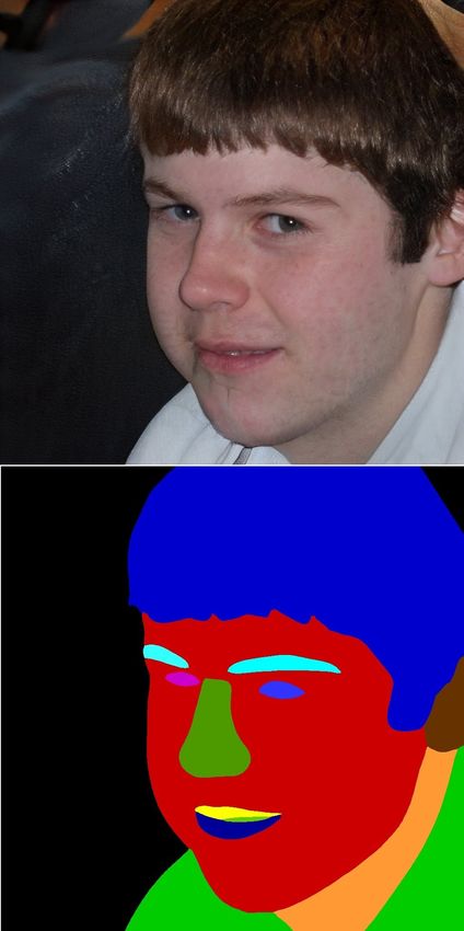
(a)                                                (b)
Figure 1: (a) Semantic projection implemented by a decoder built on top of a style-based generator as described
in Section 2.1; (b) LayerMatch scheme for pretraining a backbone to approximate the activations of a GAN
model as described in Section 3.1.

data and requires only a trained generator model, it can be used for unsupervised domain-specific
pretraining.
As a practical use-case we consider the scenario when a limited amount of labeled data is available
along with a large unlabeled dataset. This scenario is usually addressed by semi-supervised learning
methods that use both labeled and unlabeled data during training. We evaluate LayerMatch pretraining
as follows. First, a GAN model is trained on the unlabeled data, and a backbone model is pretrained
using LayerMatch with the available GAN generator. Then, a semantic segmentation model with
the LayerMatch-pretrained backbone is fine-tuned on the labeled part of the data. We perform
experiments on two datasets with high quality GAN models available (CelebA-HQ [19] and LSUN
[30]). Surprisingly, we find that LayerMatch pretraining outperforms both the standard supervised
pretraining on ImageNet and the recent semi-supervised semantic segmentation methods based on
pseudo-labeling [20] and adversarial training [11].
The rest of the paper is organized as follows. In Section 2.1 we explore semantic projections of
GAN generator and describe our experiments. In Section 3.1 we introduce the LayerMatch scheme
for unsupervised domain-specific pretraining that is based on inverting GAN generator. Section 4
describes our experiments with the models pretrained using LayerMatch. In Section 5 we discuss
related works.

2     Semantic projection of a GAN generator
Let us introduce the following notation. A typical GAN model consists of a jointly trained generator
G and a discriminator D. Generator G transforms a random latent vector l ∈ Rk into an image
Igen ∈ R3×H×W and discriminator D : R3×H×W → R classifies whether an image is real or fake.
Let us denote the activations of internal layers of G for latent vector l by Φ(l).
Semantic projection of a generator P is a mapping of the features Φ(l) onto the dense label map
L ∈ {1, . . . , C}W ×H where C is the number of classes. It can be implemented as a decoder that
takes the features from different layers of a generator and outputs the semantic segmentation result.
An example of a decoder architecture built on top of a style-based generator is shown in Figure 1 (a).

2.1   Converting semantic projection model into a segmentation model

Training procedure of a semantic projection model is shown in Algorithm 1. First, we sample a few
images using GAN generator G and store corresponding activations {Φi }, Φi = (φi1 , . . . , φik ), i =
1 . . . n of internal layers. The latent vectors are sampled from normal distribution. Then, we
manually annotate a few generated images. The decoder is trained in a supervised manner using the
segmentation masks from the previous step with corresponding intermediate generator features. We
use cross-entropy between the predicted mask and ground truth as a loss function.

                                                      2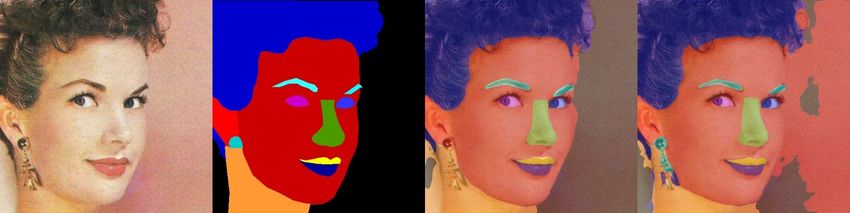
Algorithm 1: Training semantic projection model
Input: GAN model (G, D)
Output: Semantic projection model P
1 Generate n images from the random latent vectors Ii = G(li ), li ∼ N (0, σ), i = 1 . . . n and
store them along with their features {(Ii , Φi )}, i = 1 . . . n
2 Annotate the images and create semantic maps Li , i = 1 . . . n
3 Train a decoder P on pairs {(Φi , Li )}, i = 1 . . . n
Once we have trained a semantic projection model P , we can obtain pixelwise annotation for
generated images. For this purpose, we can apply P to the features produced by generator Lgen =
P (Φ). However, the features of a generator are not available for real images. Since semantic
projection alone does not allow obtaining semantic segmentation maps for real images, we propose
Algorithm 2 for converting the semantic projection model into a semantic segmentation model
applicable to real images. The intuition is that training on a large number of GAN-generated
images along with accurate annotations provided by semantic projection should result in an accurate
segmentation model.
Algorithm 2: Converting semantic projection into semantic segmentation model
Input: GAN model (G, D), semantic projection model P
Output: Semantic segmentation model S
1 Generate N images from the random latent vectors Ii = G(li ), li ∼ N (0, σ) i = 1 . . . N and
store them along with their features {(Ii , Φi )}, i = 1 . . . N
2 Compute results of semantic projection {P (Φi )}, i = 1 . . . N
3 Train semantic segmentation model S on pairs {(Φi , P (Φi ))}, i = 1 . . . N
2.2 Experiments with semantic projections
In this section we address the following questions: 1) Will a lightweight decoder be sufficient to
implement an accurate semantic projection model? 2) How many images are required to train
semantic projection to a reasonable accuracy? 3) Will the use of Algorithm 2 lead to improved
performance on real images?
Experimental protocol. We perform experiments with style-based generator [13] on two datasets
(FFHQ and LSUN-cars). In both experiments, we manually annotate 20 randomly generated images
for training the semantic projection models. For FFHQ experiment we use two classes: hair and
background. Hair is a challenging category for segmentation as it usually has difficult shape with
narrow elongated parts. For LSUN-cars we use car and background categories. We also train
DeepLabV3+ [6] model using Algorithm 2 with semantic projection models trained on 20 images. In
all experiments we use ResNet-50 as a backbone. For LSUN-cars we experiment with both ImageNet-
pretrained and randomly initialized backbones. For comparison we train a similar DeepLabV3+ model
on 20 labeled real images. 80 annotated real images are used for testing the semantic segmentation
models. Pixel accuracy and intersection-over-union (IoU) are measured for methods comparison.
Architecture of the semantic projection model. The lightweight decoder architecture for semantic
projection is shown in Figure 1. It has an order of magnitude fewer parameters compared to the
standard decoder architectures and 16 times fewer than DeepLabV3+ decoder. Each CBlock of the
decoder takes the features from corresponding SBlock of StyleGAN as an input. CBlock consists
of a 50% dropout, a convolutional and a batch normalization layers. Each RBlock of a decoder has
one residual block with two convolutional layers. The number of feature maps in each convolutional
layer of the decoder is set to 32, as wider feature maps resulted in just minor improvement in our
experiments.
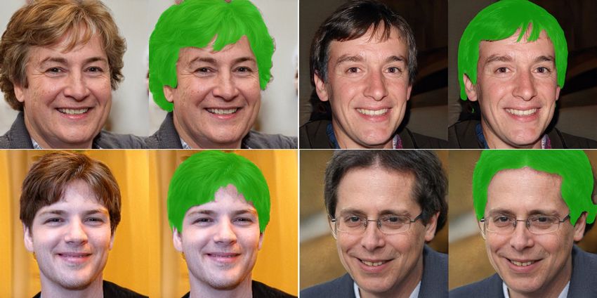
Results and discussion. Figure 2 (b) shows outputs of a semantic projection model trained on 20
synthetic images using Algorithm 1. The results of varying the size of a training set from 1 to 15
synthetic images is shown in Figure 2 (a). The test set in this experiment contains 30 manually
annotated GAN-generated images. We observe that even with a single image in training set, the
model achieves reasonable segmentation quality, and the quality grows quite slowly after 10 images.
3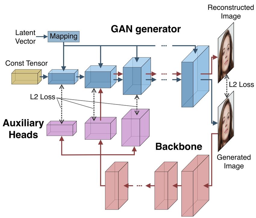
(a)                                             (b)
Figure 2: (a) - evaluation results of the semantic projection model on two classes (background and hair) with
respect to the number of images in training; (b) - outputs of semantic projection model for test images generated
by StyleGAN. Note that while the model was trained just on 20 images, it provides quite accurate segmentation.

Figure 3: Outputs of two semantic segmentation models trained with equal amount of supervision. First row -
FFHQ, second row - LSUN-cars. From left to right: input image, output of the model trained with Algorithm 2
on synthetic images, output of the model trained on the same number of real images.

                                                                ImageNet-pretrained
       Categories       Method                                                           accuracy      IoU
                                                                    backbone
                        Training on 20 labeled images                                     0.9515      0.8194
    Hair/Background                                                       +
                        Algorithm 2 with 20 labeled images                                0.9675      0.8759
                        Training on 20 labeled images                                     0.8588      0.6983
                                                                           -
                        Algorithm 2 with 20 labeled images                                0.9787      0.9408
    Car/Background
                        Training on 20 labeled images                                     0.9641      0.9049
                                                                          +
                        Algorithm 2 with 20 labeled images                                0.9862      0.9609

Table 1: Comparison of the segmentation models trained with equal amount of supervision. See text for more
details.

Next, we compare two semantic segmentation models trained with equal amount of supervision. The
first one uses Algorithm 2 with semantic projection model trained on 20 synthetic images. The second
one uses ImageNet-pretrained backbone and is trained on 20 real images. Table 1 shows quantitative
comparison of the two models. One can notice that in case when the backbone for DeepLabV3+ is
randomly initialized, the model trained with Algorithm 2 is significantly more accurate compared
to the baseline approach. When using ImageNet-pretrained backbones, Algorithm 2 leads to 6%
improvement in terms of IoU for both datasets. Figure 3 shows examples of hair and car segmentation
for real images from the test set.
Our experiments of two datasets demontrate that a lightweight decoder is sufficient to implement an
accurate semantic projection model. We observe that just a few annotated images are enough to train
semantic projection to a reasonable accuracy. The Algorithm 2 leads to improved accuracy on real
images compared to simply training a similar model with the same number of annotated images.

3    Transfer learning using generator representation

Training a semantic projection model introduced in Section 2.1 requires manual annotation of GAN-
generated images. Thus, we cannot use standard real-image datasets for comparison with other works.
Real images could potentially be embedded into the GAN latent space, but in practice this approach
has its own limitations [4]. Besides, some of the images produced by GAN generators can be hard to
label.

                                                       4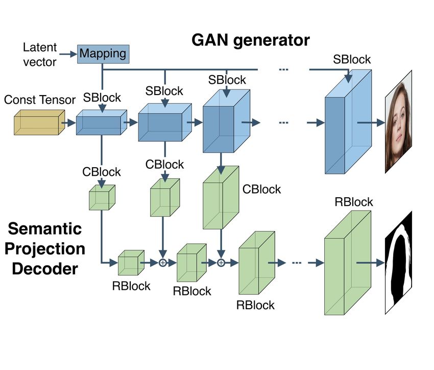
(a)                    (b)                              (c)
Figure 4: (a) - example face image with color-coded semantic annotation, (b) - t-SNE visualization of the
features of an ImageNet-pretrained backbone, (c) - similar visualization of the features learnt with LayerMatch.
In (b) and (c) each point is color-coded according to the ground truth annotation. See text for more details.

A semantic segmentation network transforms an image I ∈ R3×H×W into a segmentation map. At
the same time a GAN generator G transforms a random vector l ∈ Rk into an image Igen ∈ R3×H×W .
Obviously, the input dimensions of these two types of models do not match. Therefore, the models
trained for image generation cannot be directly applied to image segmentation. To overcome this
issue one can think of inverting a generator. Inverted GAN generators have been widely used for the
task of image manipulation [1, 4]. For this purpose, an encoder model is usually trained to predict the
latent vector from an image. Following [1, 4] we train an encoder network, but predict the activations
of a fixed GAN generator instead of the latent vector. The backbone of the trained encoder can then
be used to initialize a semantic segmentation model.

3.1   Unsupervised pretraining with LayerMatch

The scheme of the LayerMatch algorithm is shown in Figure 1 (b). We can view generator G
as a function of the latent vector l and all the intermediate activations: G = G(l, φ1 , φ2 , .., φn ),
where intermediate features themselves depend on the latent vector and all the previous features:
φi = φi (l, φ1 , φ2 , .., φi−1 ). The generated image Igen is fed to the encoder E, which tries to predict
the n specified activation tensors: Φ̂ = E(Igen ), where Φ̂ = (φ̂1 , φ̂2 , . . . , φ̂n ).
The loss function for LayerMatch training consists of two terms:
                                            L = Lrec + Lmatch ,                                             (1)

where matching loss Lmatch is the sum of the L2-losses between generated and predicted features
that penalizes difference between the outputs of the encoder and the activations of the generator:

                                                         n
                                                     1X               2
                                        Lmatch =           kφi − φ̂i k2                                     (2)
                                                     n i=1

Reconstructed image Irec is obtained by replacing random feature φm with φ̂m , where 1 ≤ m ≤ n,
and recalculating features φ˜j = φj (l, φ1 , . . . , φm−1 , φ̂m , φ̃m+1 . . . φj−1
                                                                               ˜ ), m < j ≤ n:

                              Irec = G(l, φ1 , . . . , φm−1 , φ̂m , φ̃m+1 , .., φ̃n )                       (3)

Reconstruction loss Lrec is the L2-loss between the generated image and the reconstructed image.
This loss controls that the generator produces an image which is close to the original one when
generator activations are replaced with the outputs of the backbone:
                                                                      2
                                           Lrec = kIrec − Igen k2                                           (4)

Figure 4 shows t-SNE visualizations of the features from the internal layers of two similar models.
Each point on the plots (b) and (c) represents a feature vector corresponding to a particular position
in an image. We used the activations for 5 images in this visualization. Plot (a) shows the activations
of an ImageNet-pretrained model, and the plot (b) shows activations of the model pretrained with

                                                        5
LayerMatch. One can observe that the distribution of the features learned by LayerMatch contains
    semantically meaningful clusters, while the universal features of an ImageNet-pretrained backbone
    look more scattered.

    4   Experiments with LayerMatch

    Evaluation protocol. The standard protocol for evaluation of unsupervised learning techniques
    proposed in [32] involves training a model on unlabeled ImageNet, freezing its learned representation,
    and then training a linear classifier on its outputs using all of the training set labels. This protocol
    is based on the assumption that the resulting representation is universal and applicable to different
    domains. We rather focus on domain-specific pretraining, or "specializing" the backbone to a
    particular domain. We aim at high-resolution tasks, e.g. semantic segmentation. Therefore, we apply
    a different evaluation protocol.
    We assume that we have a high-quality GAN model trained on a large unlabeled dataset from the
    domain of interest along with a limited number of annotated images from the same domain. The
    unlabeled data is used for training a GAN model, which in turn is used for pretraining the backbone
    model using LayerMatch (see Algorithm 3). The pixelwise-annotated data is later used for training a
    fixed semantic segmentation network with the pretrained backbone using a standard cross-entropy
    loss. Then, we evaluate the resulting model on a test set across the standard semantic segmentation
    metrics such as mIOU and pixel accuracy. We perform experiments with varying fraction of labeled
    data. In all our experiments we initialize the networks with ImageNet-pretrained backbones.

    Algorithm 3: Training semantic projection model
    Input: GAN model (G, D) trained on a large unlabeled dataset, a small labeled dataset
           (Ij , Lj ), j = 1 . . . n
    Output: Semantic segmentation model S
1      Generate N images from the random latent vectors Ii = G(li ), li ∼ N (0, σ), i = 1 . . . N and
        store them along with their features {(Ii , Φi )}, i = 1 . . . N
2      Train the backbone using LayerMatch using the pairs {(Ii , Φi )}, i = 1 . . . N
3      Train a semantic segmentation model S on the labeled part of the data {(Ij , Lj )}, j = 1 . . . n

    Comparison with prior work. For all compared methods we use the same network architectures
    differing only in training procedure and loss functions used. The first baseline uses a standard
    ImageNet-pretrained backbone without domain-specific pretraining. The semantic segmentation
    model is trained using available annotated data and does not use the unlabeled data.
    The other two baselines are recent semi-supervised segmentation methods using both labeled and
    unlabeled data during training. In the experiments with these methods we used exactly the same
    amount of both labeled and unlabeled data as for LayerMatch. Namely, for the experiments with
    Celeba-HQ we used both the unlabeled part of CelebA and the FFHQ dataset, that was used for GAN
    training. For the experiments with LSUN-church all the unlabeled data in LSUN-church dataset was
    used during training.
    The first semi-supervised segmentation method that we use for comparison is based on pseudo-
    labeling [20]. Unlabeled data is augmented by generating pseudo-labels using the network predictions.
    Only the pixels with high-confidence pseudo-labels are used as ground truth for training. The second
    one is an adversarial semi-supervised segmentation approach [11]. In this method the segmentation
    network is supervised by both the standard cross-entropy loss with the ground truth label map
    and the adversarial loss with the discriminator network. In our experiments we used the official
    implementation provided by the authors, and changed only the backbone.
    Datasets. Celeba-HQ [19] contains 30,000 high-resolution face images selected from the CelebA
    dataset [22], each image having a segmentation mask with the resolution of 512x512 and 19 classes
    including all facial components and accessories such as skin, nose, eyes, eyebrows, ears, mouth,
    lips, hair, hat, eyeglass, earring, necklace, neck, cloth, and background. We use a StyleGAN2
    model trained on FFHQ dataset provided in [15] that has a FID measure 3.31 and PPL 125. In the
    experiments with Celeba-HQ we vary the fraction of labeled data from 1/1024 to the full dataset.

                                                       6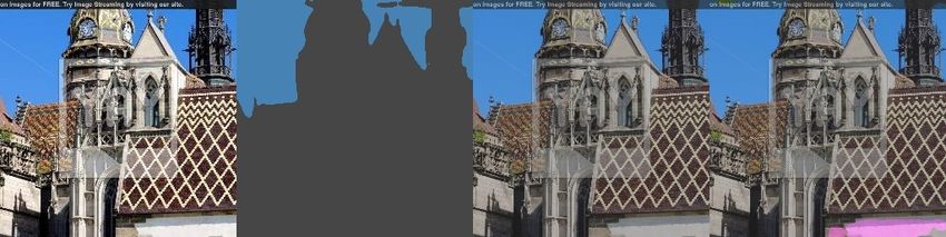
(a)                                          (b)
Figure 5: Comparison of the models trained with Algorithm 3 to semi-supervised segmentation methods for a
varying number of annotated samples. (a) - FFHQ+CelebA-HQ dataset. (b) - LSUN-church dataset

LSUN-church [31] contains 126,000 images of churches of 256x256 resolution. We have selected top
10 semantic categories that occupy more than 1% of image area, namely road, vegetation, building,
sidewalk, car, sky, terrain, pole, fence, wall. We use a StyleGAN2 model provided in [15] that has a
FID measure 3.86 and PPL 342. As LSUN dataset does not contain pixelwise annotation, we take the
outputs of the Unified Scene Parsing Network [29] as ground truth in this experiment similarly to
[4]. In the experiments with Celeba-HQ we vary the fraction of labeled data from 1/4096 to the full
dataset.
Implementation details. HRNet [28] is used as an encoder architecture. We add K auxiliary heads
for each of K activations that we want to predict (see Figure 1 (b)). After training, auxiliary heads
are discarded and only the pretrained backbone is used for transfer learning, similar to ImageNet
pretraining. For pretraining the encoder we use Adam optimizer with the learning rate 10−4 and
the cosine learning rate decay. We use source code from HRNet repository for training semantic
segmentation networks.
Results and discussion. Figure 5 shows the comparison of the proposed LayerMatch pretraining
scheme to 3 baseline methods across 2 datasets with varying fraction of annotated data. Pseudo-
labeling is applicable in case when some part of the dataset is unlabelled.
One can see that LayerMatch pretraining shows significantly higher IoU compared to the baseline
methods on Celeba-HQ (see Figure 5 (a)) for any fraction of the labeled data. For LSUN-church it
shows higher accuracy compared to other methods in cases when up to 1/512 of the data is annotated.
Figure 6 shows qualitative comparison of the model pretrained with LayerMatch to the standard
ImageNet pretraining on Celeba-HQ when trained with 1/512 of annotated data. The difference
between two models is quite noticeable for both CelebA-HQ and for LSUN-church. Table 2 shows
category-wise results for all four compared models trained with 1/512 of labeled data. LayerMatch
pretraining leads to significant accuracy improvement for the eyeglasses category.
Overall, LayerMatch pretraining leads to improved results in semi-supervised learning scenario
compared to both simple ImageNet pretraining and to semi-supervised segmentation methods. Lower
accuracy for larger fraction of annotated datasets on LSUN-church can be attributed to lower quality
of LSUN-church GAN generator compared to Celeba-HQ GAN generator. Another possible reason
for this effect may be the imperfect annotation of both training and test data, which may lead to
inaccuracies in evaluation.

5   Related work
Several works consider generative models for unsupervised pretraining [23, 18, 8, 9]. One of the
approaches [27] uses representation learnt by a discriminator. Another line of research extends GAN
to bidirectional framework (BiGAN) by introducing an auxiliary encoder branch that predicts the
latent vector from a natural image [8, 9]. The encoder learnt via BiGAN framework can be used
as feature extractor for downstream tasks [9]. The use of GANs as universal feature extractors has
severe limitations. First, GANs are not always capable of learning a multimodal distribution as they
tend to suffer from mode collapse [21]. The trade-off between GAN precision and recall is still

                                                   7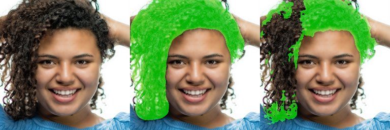
background

                                                                  eye glasses

                                                                                                                   right brow
                                                                                                       left brow

                                                                                                                                                               upper lip
                                                                                                                                                                           lower lip
                                                                                           right eye

                                                                                                                                                                                                         necklace
                                                                                                                                           right ear

                                                                                                                                                                                              earrings
                                                                                left eye
                       pixAcc

                                                                                                                                left ear

                                                                                                                                                       mouth
                                mIoU

                                                                                                                                                                                                                           cloth
                                                                                                                                                                                                                    neck
                                                           nose
                                                    skin

                                                                                                                                                                                       hair
                                                                                                                                                                                              hat
      Method
   ImageNet only       .92      .62    .89          .89    .87    .01           .75        .77         .67         .68          .71        .72         .76     .74         .79         .87    0.   .34   0.         .77    .62
 AdvSemiSeg [11]       .91      .62    .89          .89    .85    .14           .75        .77         .66         .66          .71        .70         .77     .73         .78         .86    0.   .29   0.         .75    .59
Pseudo-labeling [20]   .92      .63    .89          .90    .86    .01           .77        .78         .71         .70          .73        .72         .79     .75         .79         .86    0.   .33   0.         .77    .58
    LayerMatch         .93      .67    .90          .91    .87    .68           .78        .78         .70         .69          .75        .74         .79     .76         .80         .87    0.   .34   0.         .80    .64

Table 2: Comparison of segmentation models trained on CelebA-HQ dataset with equal amount of supervision.
Notice that LayerMatch provides better results for almost all categories and improves the IoU for eye glasses
category by several times.

Figure 6: Test results. First row: CelebA-HQ, 1/512, second row: LSUN-church, 1/512. From left to right:
input image, LayerMatch pretraining, ImageNet pretraining only.

difficult to control [17]. Besides, training a GAN on a large dataset of high-resolution images requires
an extremely large computational budget, which makes ImageNet-scale experiments prohibitively
expensive. Our approach differs from this line of work, as we use a GAN to specialize a model
to a particular domain rather than trying to obtain universal feature representations. We explore
the representation of a GAN generator that, to the best of our knowledge, has not been previously
considered for transfer learning.
Bau et al. [3] show that activations of a generator are highly correlated with semantic segmentation
masks for the generated image. One of the means for analysis of latent space and internal representa-
tion of a generator is latent embedding, i.e. finding a latent vector that corresponds to a particular
image. Several methods for embedding images into GAN latent space have been proposed [15, 4, 1],
bringing interesting insights about generator representations. For instance, it allowed to demonstrate
that some of semantic categories are missing systematically in GAN-generated images [4]. Similarly
to these works we invert a GAN generator using both feature approximation and image reconstruction
losses, although we do not aim at reconstructing the latent code, and only approximate the activations
of the layers of a generator.
While image-level classification has been extensively studied in a semi-supervised setting, dense
pixel-level classification with limited data has only drawn attention recently. Most of the works on
semi-supervised semantic segmentation borrow the ideas from semi-supervised image classification
and generalize them on high-resolution tasks. [11] adopt an adversarial learning scheme and propose
a fully convolutional discriminator that learns to differentiate ground truth label maps from proba-
bility maps of segmentation predictions. [25] use two network branches that link semi-supervised
classification with semi-supervised segmentation including self-training.

6   Conclusion
We study the use of GAN generators for the task of learning domain-specific representations. We show
that the representation of a GAN generator can be easily projected onto semantic segmentation map
using a lightweight decoder. Then, we propose LayerMatch scheme for unsupervised domain-specific
pretraining that is based on approximating the generator representation. We present experiments in
semi-supervised learning scenario and compare to recent semi-supervised semantic segmentation
methods.

                                                                                            8
References
[1] Abdal, R., Qin, Y., and Wonka, P. (2019). Image2stylegan: How to embed images into the stylegan latent
   space? In Proceedings of the IEEE International Conference on Computer Vision, pages 4432–4441.

[2] Arjovsky, M., Chintala, S., and Bottou, L. (2017). Wasserstein gan. arXiv preprint arXiv:1701.07875.

[3] Bau, D., Zhu, J.-Y., Strobelt, H., Zhou, B., Tenenbaum, J. B., Freeman, W. T., and Torralba, A. (2018). Gan
   dissection: Visualizing and understanding generative adversarial networks. arXiv preprint arXiv:1811.10597.

[4] Bau, D., Zhu, J.-Y., Wulff, J., Peebles, W., Strobelt, H., Zhou, B., and Torralba, A. (2019). Seeing what
   a gan cannot generate. In Proceedings of the IEEE International Conference on Computer Vision, pages
   4502–4511.

[5] Brock, A., Donahue, J., and Simonyan, K. (2018). Large scale gan training for high fidelity natural image
   synthesis. arXiv preprint arXiv:1809.11096.

[6] Chen, L.-C., Zhu, Y., Papandreou, G., Schroff, F., and Adam, H. (2018). Encoder-decoder with atrous
   separable convolution for semantic image segmentation. In ECCV.

[7] Chen, X., Duan, Y., Houthooft, R., Schulman, J., Sutskever, I., and Abbeel, P. (2016). Infogan: Interpretable
   representation learning by information maximizing generative adversarial nets. In Advances in neural
   information processing systems, pages 2172–2180.

[8] Donahue, J., Krähenbühl, P., and Darrell, T. (2016). Adversarial feature learning. arXiv preprint
   arXiv:1605.09782.

[9] Donahue, J. and Simonyan, K. (2019). Large scale adversarial representation learning. In Advances in
   Neural Information Processing Systems, pages 10541–10551.

[10] Goodfellow, I., Pouget-Abadie, J., Mirza, M., Xu, B., Warde-Farley, D., Ozair, S., Courville, A., and
   Bengio, Y. (2014). Generative adversarial nets. In Advances in neural information processing systems, pages
   2672–2680.

[11] Hung, W.-C., Tsai, Y.-H., Liou, Y.-T., Lin, Y.-Y., and Yang, M.-H. (2018). Adversarial learning for
   semi-supervised semantic segmentation. arXiv preprint arXiv:1802.07934.

[12] Karras, T., Aila, T., Laine, S., and Lehtinen, J. (2017). Progressive growing of gans for improved quality,
   stability, and variation. arXiv preprint arXiv:1710.10196.

[13] Karras, T., Laine, S., and Aila, T. (2018). A style-based generator architecture for generative adversarial
   networks. arXiv preprint arXiv:1812.04948.

[14] Karras, T., Laine, S., and Aila, T. (2019a). A style-based generator architecture for generative adversarial
   networks. In Proceedings of the IEEE Conference on Computer Vision and Pattern Recognition, pages
   4401–4410.

[15] Karras, T., Laine, S., Aittala, M., Hellsten, J., Lehtinen, J., and Aila, T. (2019b). Analyzing and improving
   the image quality of stylegan. arXiv preprint arXiv:1912.04958.

[16] Kingma, D. P. and Dhariwal, P. (2018). Glow: Generative flow with invertible 1x1 convolutions. In
   Advances in Neural Information Processing Systems, pages 10215–10224.

[17] Kynkäänniemi, T., Karras, T., Laine, S., Lehtinen, J., and Aila, T. (2019). Improved precision and recall
   metric for assessing generative models. In Advances in Neural Information Processing Systems, pages
   3929–3938.

[18] Larsen, A. B. L., Sønderby, S. K., Larochelle, H., and Winther, O. (2015). Autoencoding beyond pixels
   using a learned similarity metric. arXiv preprint arXiv:1512.09300.

[19] Lee, C.-H., Liu, Z., Wu, L., and Luo, P. (2019). Maskgan: towards diverse and interactive facial image
   manipulation. arXiv preprint arXiv:1907.11922.

[20] Lee, D.-H. (2013). Pseudo-label: The simple and efficient semi-supervised learning method for deep neural
   networks. In Workshop on challenges in representation learning, ICML, volume 3, page 2.

[21] Liu, K., Tang, W., Zhou, F., and Qiu, G. (2019). Spectral regularization for combating mode collapse in
   gans. In Proceedings of the IEEE International Conference on Computer Vision, pages 6382–6390.

                                                        9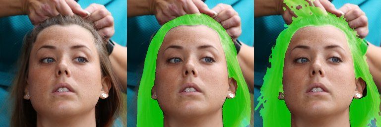
[22] Liu, Z., Luo, P., Wang, X., and Tang, X. (2015). Deep learning face attributes in the wild. In Proceedings
   of International Conference on Computer Vision (ICCV).

[23] Makhzani, A., Shlens, J., Jaitly, N., Goodfellow, I., and Frey, B. (2015). Adversarial autoencoders. arXiv
   preprint arXiv:1511.05644.
[24] Mescheder, L., Geiger, A., and Nowozin, S. (2018). Which training methods for gans do actually converge?
   arXiv preprint arXiv:1801.04406.

[25] Mittal, S., Tatarchenko, M., and Brox, T. (2019). Semi-supervised semantic segmentation with high-and
   low-level consistency. IEEE Transactions on Pattern Analysis and Machine Intelligence.

[26] Miyato, T., Kataoka, T., Koyama, M., and Yoshida, Y. (2018). Spectral normalization for generative
   adversarial networks. arXiv preprint arXiv:1802.05957.

[27] Radford, A., Metz, L., and Chintala, S. (2015). Unsupervised representation learning with deep convolu-
   tional generative adversarial networks. arXiv preprint arXiv:1511.06434.

[28] Sun, K., Zhao, Y., Jiang, B., Cheng, T., Xiao, B., Liu, D., Mu, Y., Wang, X., Liu, W., and Wang, J. (2019).
   High-resolution representations for labeling pixels and regions. arXiv preprint arXiv:1904.04514.
[29] Xiao, T., Liu, Y., Zhou, B., Jiang, Y., and Sun, J. (2018). Unified perceptual parsing for scene understanding.
   In Proceedings of the European Conference on Computer Vision (ECCV), pages 418–434.

[30] Yu, F., Seff, A., Zhang, Y., Song, S., Funkhouser, T., and Xiao, J. (2015a). Lsun: Construction of a
   large-scale image dataset using deep learning with humans in the loop. arXiv preprint arXiv:1506.03365.

[31] Yu, F., Zhang, Y., Song, S., Seff, A., and Xiao, J. (2015b). Lsun: Construction of a large-scale image
   dataset using deep learning with humans in the loop. arXiv preprint arXiv:1506.03365.

[32] Zhang, R., Isola, P., and Efros, A. A. (2016). Colorful image colorization. In European conference on
   computer vision, pages 649–666. Springer.

                                                        10
You can also read