Analyzing Restricted Mean Survival Time Using SAS/STAT
←
→
Page content transcription
If your browser does not render page correctly, please read the page content below
Paper SAS3013-2019

            Analyzing Restricted Mean Survival Time Using SAS/STAT®

                            Changbin Guo and Yu Liang, SAS Institute Inc., Cary, NC

ABSTRACT
Survival analysis handles time-to-event data. Classical methods, such as the log-rank test and the Cox proportional
hazards model, focus on the hazard function and are most suitable when the proportional hazards assumption holds.
When it does not hold, restricted mean survival time (RMST) methods often apply. The RMST is the expected survival
time subject to a specific time horizon, and it is an alternative measure to summarize the survival profile. RMST-based
inference has attracted attention from practitioners for its capability to handle nonproportionality. This paper introduces
RMST methods in SAS/STAT® software: you can now use the RMSTREG procedure to fit linear and log-linear
models, and you can use the RMST option in PROC LIFETEST to estimate the restricted mean survival time and
make comparisons between groups. The paper discusses the rationale behind the RMST-based approach, outlines
its recent development, and uses examples to illustrate real-world applications of the RMSTREG and LIFETEST
procedures.

INTRODUCTION
The proportional hazards (PH) assumption plays an important role in survival data analysis. It is the basis of the
popular Cox proportional hazards model. The widely applied log-rank test is equivalent to a score test of the PH model
and achieves its highest power when the PH assumption is satisfied. However, practitioners have encountered various
situations in which the PH assumption is questionable or simply untenable. Although it is possible to modify the
classical methods to accommodate certain non-PH settings, solutions are rather limited, and often they are formulated
at the expense of meaningful interpretations (Uno et al. 2014).
There are a handful of assumption-free measures of the survival outcome. For example, the mean and the median
of the event time have been commonly used as summary statistics, and the differences or ratios of these quantities
are often used to measure group effects. Censoring has posed special challenges that limit their usages. For
example, if the last observation is censored, then you cannot reliably estimate the mean; and when not enough events
occur, the median can be inestimable. The survival rate at a specified time is another commonly used summary
statistic. Although it can be less problematic than the mean or median, it does not provide an overall summary of the
time-to-event outcome.
The restricted mean survival time (RMST), sometimes called the restricted mean event time, is an alternative measure
that is more often reliably estimable than the mean and median of the event time in certain situations. Also, it provides
a summary of the whole survival curve up to a time horizon, in contrast to the survival rate at a specified time (Royston
and Parmar 2013; Uno et al. 2014; Trinquart et al. 2016). The RMST has attracted practitioners for its straightforward
interpretation and its capability to deal with nonproportional hazards. When two survival curves cross, the difference
in the RMST between two groups still provides information about efficacy in a clinical trial, whereas the log-rank test
fails to detect the significance and the hazard ratio becomes meaningless.
Starting in SAS/STAT 15.1, new, dedicated features are available for analyzing the RMST. You can use the RMST
option in the LIFETEST procedure to perform nonparametric analysis with respect to the RMST. You can also use the
new RMSTREG procedure to fit linear and log-linear models of the RMST.
This paper first presents the limitations of the classical hazard-based methods. It then introduces the RMST as an
alternative measure and uses real-world data examples to illustrate how to perform nonparametric analysis with
respect to the RMST. The next four sections focus on regression modeling and show how you can use pseudovalue
regression and inverse probability censoring weighting techniques to fit the linear and log-linear models and make
model-based inferences. Differences and connections with classical methods are also discussed.

                                                            1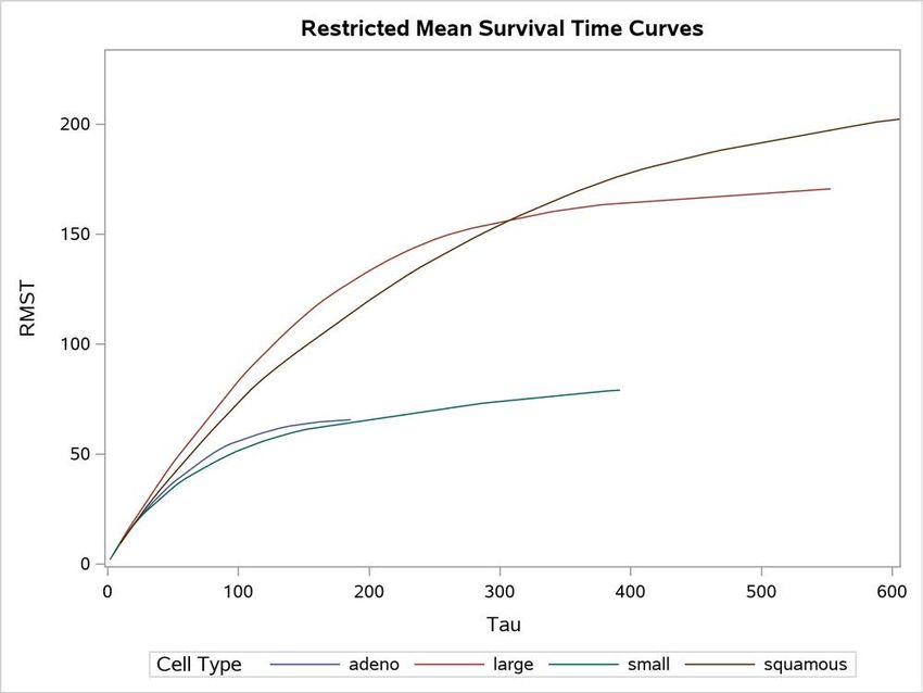
LIMITATIONS OF HAZARD-BASED METHODS
In practical survival analysis, methods such as the log-rank test and Cox regression have become standard tools.
Their use is warranted when the assumption of proportional hazards (PH) holds. In this case, the log-rank test is more
powerful than other nonparametric tests, and the estimated effects in a Cox regression can be interpreted in terms of
hazard ratios. However, the PH assumption is often not satisfied in real-world applications, and this can make the
results unusable.
A typical violation of the PH assumption occurs when the two survival curves cross. This implies that the corresponding
hazard functions would also cross. Because the log-rank statistic is essentially a weighted sum of the hazard function
over time, the log-rank test loses much of its power to detect the true difference in survival. Results from the Cox PH
regression have the same problem. As the true hazard ratio changes over time, the estimated hazard ratio from the
fitted model ends up being a weighted average of the time-varying hazard ratios and can be interpreted as such. The
problem is that the weights depend on the underlying survival and censoring distributions and therefore cannot be
generalized straightforwardly.
RESTRICTED MEAN SURVIVAL TIME AS AN ALTERNATIVE MEASURE
Definition
Let T be a nonnegative random variable that represents the failure time of an individual from a homogeneous
population. The survivor function (also known as the survival function) of T is defined as
S.t / D Pr.T > t/
Assume that
is a prespecified time point of interest. Let R be the minimum of T and
:
R D T ^
D min.T;
/
The restricted mean survival time is defined as the expected value of R :
RMST.
/ D E.R/ D EŒmin.T;
/
It can be evaluated by the area under the survivor function over Œ0;
as
Z
RMST.
/ D S.u/du
0
The restricted mean time lost (RMTL) is defined as the expected value of
R:
Z
RMTL.
/ D E.
R/ D
EŒmin.T;
/ D Œ1 S.u/du
0
Statistical Analysis and Software
You can essentially make the same types of statistical inferences on the RMST as you can in the classical setting
where the survival and hazard functions are the primary interests. Table 1 summarizes various inference objectives in
the classical setting and the RMST setting.
Table 1 Inference Objectives in Classical and RMST Settings
Task Classical Setting RMST Setting
Estimation S.t/ RMST.
/
H0 : S1 .t/ D S2 .t / H0 : RMST1 .
/ D RMST2 .
/
Testing
H1 : S1 .t/ ¤ S2 .t / H1 : RMST1 .
/ ¤ RMST2 .
/
PH: h.t/ D h0 .t / exp.x0ˇ/ Linear: RMST.
/ D ˇ0 C x0ˇ
Regression
AFT: log.t / D ˇ0 C x0ˇ C Log-linear: log.RMST.
// D ˇ0 C x0ˇ
SAS/STAT software is well developed in the classical setting. PROC LIFETEST traditionally focuses on the estimating
and testing tasks for the survival functions and supports nonparametric methods such as the Kaplan-Meier estimator
2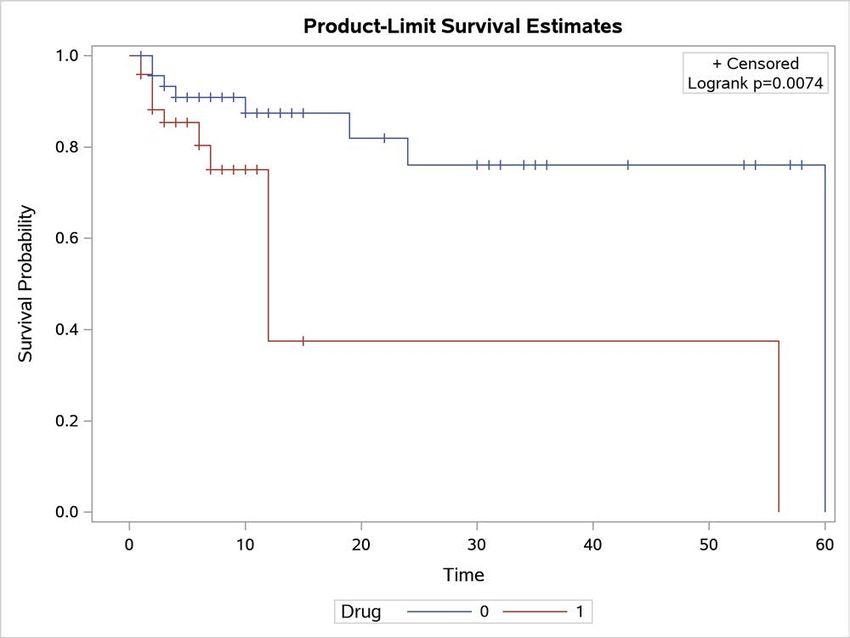
and the log-rank test. The assumption-free nonparametric methods for the RMST extend these classical methods. In
SAS/STAT 15.1, you can use the new RMST option in the LIFETEST procedure to estimate and compare the RMST.
The proportional hazards (PH) model and the accelerated failure time (AFT) model are popular choices for analyzing
time-to-event data. In SAS/STAT, the PHREG procedure fits primarily the Cox PH model to right-censored data but
also fits other types of PH models. The LIFEREG procedure can fit parametric AFT models to arbitrarily censored
data. A key difference between the two procedures is that the Cox PH model does not assume a particular form on
the baseline hazard function h0 .t/, whereas the AFT model assumes that the error term follows certain parametric
distributions, such as Weibull or exponential. The new RMSTREG procedure in SAS/STAT 15.1 provides regression
modeling capabilities for the RMST setting and fits generalized linear models such as linear and log-linear models to
right-censored data. Table 2 summarizes the key features of these procedures.
Table 2 Survival Modeling Procedures
Procedure Focus Model Type Estimation Method
PROC LIFEREG Time to event Accelerated failure time models Likelihood
PROC PHREG Hazard function Proportional hazards models Partial likelihood
PROC RMSTREG Restricted mean survival time Generalized linear models Estimating equations
It is possible to estimate RMST from a classical survival model, such as the Cox proportional hazards model (Zucker
1998), but the process is complex and difficult to extend. PROC RMSTREG avoids this difficulty by using generalized
linear modeling techniques to directly model the RMST. This approach has the double advantage of making inferences
on the results straightforward and providing all the machinery of generalized linear model comparisons for studying
RMST effects.
NONPARAMETRIC ANALYSIS USING PROC LIFETEST
The new methods of analyzing the RMST in the LIFETEST procedure focus on nonparametric estimation and group
comparisons of the RMST. This section briefly presents these methods.
Estimating the RMST
Let t1 < t2 < < tD represent distinct event times. For each i D 1; : : : ; D , let Yi be the number of surviving units
(the size of the risk set) just prior to ti , and let di be the number of units that fail at ti .
The Kaplan-Meier (product-limit) estimate of the survivor function at ti is the cumulative product
i
Y dj
SO .ti / D 1
Yj
j D1
If the largest observed time is uncensored, the estimated mean survival time is
D
X
O D O i
S.t 1 /.ti ti 1/
i D1
where t0 is defined to be 0.
RMST.
/ is estimated by
2
Z
N
X
RMST.
/ D O
S .t/dt D O i
S.t 1 /.ti ti 1/ C SO .tN /.
tN /
0 i D1
where N is the number of ti values that are less than
.
The restricted mean time lost (RMTL) is estimated by RMTL.
/ D
2 2
RMST.
/.
2 2
The standard error of RMST.
/ or RMTL.
/ is estimated as
v
u N
u m X di A2i
O D t
m 1 Yi .Yi di /
iD1
3where
N
Z
X
Ai D O
S.t/dt D O j /.tj C1
S.t tj / C SO .tN /.
tN /
ti j Di
N
X
m D dj
j D1
Comparing the RMST between Groups
Let K be the number of groups. Let Sk .t / be the underlying survivor function of the k th group, k D 1; : : : ; K .
Assume that
is a prespecified time point of interest and Sk .
/ > 0. The following methods are presented in terms of
RMST.
/, but they also extend to the analysis of RMTL.
/.
The null and alternative hypotheses to be tested are
H0 W RMST1 .
/ D RMST2 .
/ D D RMSTK .
/
versus
H1 W at least one of the RMSTk .
/’s is different
2 2 2 2
Let RMST.
/ D ŒRMST1 .
/; RMST2 .
/; : : : ; RMSTK .
/T be the vector of estimated RMSTs for the K groups.
Let † 2
O be the estimated covariance matrix for R MST.
/. It is a diagonal matrix, and the j th diagonal element is O , 2
2
j
which is the estimated variance of RMST .
/. j
Let D be a .K 1/ K matrix whose j th row is ej ej C1 , where ej is a K -dimensional vector whose j th element
is 1 and whose other elements are 0. The test statistic is computed as
2 O T / D RMST.
/
.RMST.
//T D T .D †D 2
Under the null hypothesis H0 , this K -sample test statistic has approximately a chi-square distribution with degrees of
freedom equal to the rank of D †DO T.
EXAMPLE OF NONPARAMETRIC ANALYSES
This example uses real-world data to demonstrate how you can perform nonparametric analyses of the RMST. The
data, which are presented in Appendix I of Kalbfleisch and Prentice (1980), are coded in the following DATA step.
The response variable, SurvTime, is the survival time in days of a lung cancer patient. The covariates are Cell
(type of cancer cell), Therapy (type of therapy: standard or test), Prior (prior therapy: 0=no, 10=yes), Age (age in
years), DiagTime (time in months from diagnosis to entry into the trial), and Kps (performance status). The censoring
indicator variable Censor is created from the data; the value 1 indicates a censored time, and the value 0 indicates an
event time. Because there are only two types of therapy, an indicator variable, Treatment, is created for therapy type;
the value 0 indicates standard therapy, and the value 1 indicates test therapy.
data VALung;
drop check m;
retain Therapy Cell;
infile cards column=column;
length Check $ 1;
label SurvTime='Failure or Censoring Time'
Kps='Karnofsky Index'
DiagTime='Months till Randomization'
Age='Age in Years'
Prior='Prior Treatment?'
Cell='Cell Type'
Therapy='Type of Treatment'
Treatment='Treatment Indicator';
4... more lines ...
52 60 4 45 0 164 70 15 68 10 19 30 4 39 10 53 60 12 66 0
15 30 5 63 0 43 60 11 49 10 340 80 10 64 10 133 75 1 65 0
111 60 5 64 0 231 70 18 67 10 378 80 4 65 0 49 30 3 37 0
;
The following statements use PROC LIFETEST to perform analyses of the restricted mean survival time (RMST) and
restricted mean time lost (RMTL) in addition to the standard analyses:
ods graphics on;
proc lifetest data=VALung plots=(rmst rmtl s) rmst rmtl(tau=90) maxtime=600;
time SurvTime*Censor(1);
strata Cell;
run;
ods graphics off;
The RMST and RMTL options estimate the restricted mean survival time and the restricted mean time lost, respectively.
The variable Cell is specified in the STRATA statement to compute the RMST for each type of cancer cell. ODS
Graphics must be enabled for graphs to be produced. Graphical displays of the RMST and RMTL curves are requested
through the PLOTS= option in the PROC LIFETEST statement. Because of a few large survival times, a MAXTIME=
option value of 600 is used to set the upper limit of the time axis; that is, the time horizon in the plots extends from 0 to
a maximum of 600 days.
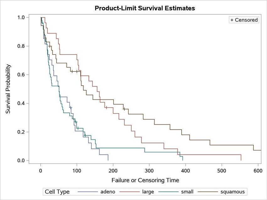
The graph of the Kaplan-Meier curves is shown in Figure 1.
Figure 1 Survival Curves
5Figure 2 displays the
value that the RMST analysis uses. If you omit the TAU= option, PROC LIFETEST uses the
smallest value among the largest observed times across the strata as the
value.
Figure 2 RMST Analysis Information
RMST
Analysis
Information
Tau 186
Figure 3 displays the RMST estimates for the four cell types.
Figure 3 RMST Estimates
RMST Estimates
Standard
Stratum Cell Type Estimate Error
1 adeno 65.55556 9.9303
2 large 128.0370 11.9858
3 small 64.20647 8.2859
4 squamous 113.8040 12.3703
Figure 4 displays information about the RMTL analysis. A
value of 90 is shown; this is the value that is specified in
the TAU= option.
Figure 4 RMTL Analysis Information
RMTL
Analysis
Information
Tau 90
Figure 5 displays the RMTL estimates for the four cell types at
D 90.
Figure 5 RMTL Estimates at
D 90
RMTL Estimates
Standard
Stratum Cell Type Estimate Error
1 adeno 36.54321 6.3206
2 large 14.33333 4.9560
3 small 41.27083 4.6763
4 squamous 22.99365 5.6430
The graph of the estimated RMST curves is shown in Figure 6. These curves exhibit a behavior similar to that of the
survival curves in Figure 1: the adeno cell curve and the small cell curve are much closer to each other than they are
to the large cell curve or the squamous cell curve. The shapes of the large cell curve and the squamous cell curve are
quite different, although the RMST in both curves increases more rapidly than the RMST in the adeno and small cell
curves. The RMST in the squamous cell curve initially increases less rapidly than the RMST in the large cell curve,
but the roles are reversed in the later period.
6Figure 6 RMST Curves
The graph of the estimated RMTL curves is displayed in Figure 7. Again, the adeno cell curve and the small cell curve
are much closer to each other and farther away from the large cell and squamous cell curves.
7Figure 7 RMTL Curves
Results of the homogeneity test for the RMST across cell types are given in Figure 8. The table displays the
approximate chi-square statistic, degrees of freedom, and p -value. The test results provide strong evidence that the
RMSTs for the four types of cancer cells are not the same (p < 0.0001).
Figure 8 Homogeneity Tests across Cell Types
RMST Test of Equality
Source Chi-Square DF Pr > ChiSq
Strata 28.4427 3Figure 9 All Paired Comparisons
The LIFETEST Procedure
Restricted Mean Survival Time Comparisons
Adjustment for Multiple Comparisons: Sidak
Pr > ChiSq
Stratum Standard
Comparison Difference Error Chi-Square Unadjusted Adjusted
adeno large -62.4815 15.5650 16.1141can interpret the effects in terms of ratios in the RMST. Both linear and log-linear models are special cases of the
generalized linear models (Nelder and Wedderburn 1972).
Let Di be the response variable for the i th observation. The quantity xi is a column vector of covariates, or explanatory
variables, for observation i that is known from the experimental setting and is considered to be fixed, or nonrandom.
The expected value of Di , denoted by i , is
i D EŒDi jxi
Under the specification of generalized linear models (Nelder and Wedderburn 1972), i is related to a linear predictor
through a monotone and differentiable link function g,
g.i / D x0i ˇ
where ˇ is an unknown parameter vector and another column can be added to xi for an intercept effect.
Assume that
is a prespecified time point of interest. Let Ti be the time-to-event variable for the i th subject. The
subject-specific RMST at
is defined by RMSTi .
/ D EŒmin.Ti ;
/ and can be conveniently modeled via a
generalized linear model as
gŒRMSTi .
/ D x0i ˇ
Under the natural logarithm link g./ D log./, the model is
logŒRMSTi .
/ D x0i ˇ
Under the identity or linear link, the model is
RMSTi .
/ D x0i ˇ
The RMSTREG procedure analyzes time-to-event data by using regression with respect to the restricted mean survival
time. It provides you with two methods to fit these models: the pseudovalue regression method (Andersen, Hansen,
and Klein 2004) and the inverse probability censoring weighting (IPCW) method (Tian, Zhao, and Wei 2014). Both
methods are generic approaches for fitting regression models to censored data, and you can apply them to the RMST
setting. But the methods have their differences. The pseudovalue regression method assumes that only the censoring
is noninformative to the survival outcomes and treats the censoring distribution as a nuisance in the estimation. On
the other hand, the IPCW technique further assumes that the censoring distribution can be properly estimated and
uses the estimates as weights explicitly in the estimation process. This feature allows the IPCW method to deal with
nonhomogeneous censoring, so it can be more efficient in those settings. However, the downside is that the IPCW
method requires the censoring distribution to be correctly estimated. The following two sections discuss these two
estimation methods in detail and present examples to illustrate how you can use them in PROC RMSTREG.
PSEUDOVALUE REGRESSION
Pseudovalue regression is a generic method of fitting generalized linear models to time-to-event data (Andersen,
Klein, and Rosthøj 2003). This section describes how the method works and how you can apply it to analyze models
of the RMST.
Let D1 ; : : : ; Dn be independent and identically distributed quantities that might be random variables or vectors of
variables. Let D EŒf .Di / for some function f ./. Suppose that O is an unbiased estimator of .
Let x1 ; : : : ; xn be independent and identically distributed samples of covariates, and define the conditional expectation
of f .Di / given by xi as
i D EŒf .Di /jxi
The i th pseudo-observation of is computed as
Oi D nO .n 1/O i
where O i
is the jackknife leave-one-out estimator for based on fDj W j ¤ i g.
The generalized linear model (Nelder and Wedderburn 1972) for assumes
g.i / D x0i ˇ
10where g./ is a suitable link function. Note that another column can be added to Xi for an intercept effect.
Using pseudo-observations, you can estimate the regression parameters ˇ by solving the following estimating
equations,
n n
@i 0
X X
U.ˇ/ D Ui .ˇ/ D Vi 1
Oi i D0
@ˇ
iD1 i D1
where Vi is a working covariance matrix.
Let ˇO be the solution of the estimating equations. You can use a sandwich estimator to estimate the variance-
covariance matrix of ˇO . It takes the form
†e D I0 1 I1 I0 1
O and is given by
I0 1 is the model-based estimator of Cov.ˇ/
n
X @i 0 1 @i
I0 D Vi
@ˇ @ˇ
i D1
O and is computed as
I1 1 is the empirical estimator of Cov.ˇ/
n
X
I1 D O 0 Ui .ˇ/
Ui .ˇ/ O
i D1
Andersen, Hansen, and Klein (2004) proposed using pseudovalue regression to analyze RMST models. Assume
that
is a prespecified time point of interest. Let Ti be the time-to-event variable for the i th subject. You can use
pseudovalue regression to fit the RMST models by letting
i D RMSTi .
/ D E.Ti ^
jxi /
i D RMSTi .
/ g.u/ D log.u/
Vi D
1 g.u/ D u
2
Because the nonparametric estimator RMST.
/ based on the Kaplan-Meier estimator is unbiased, you can use it in
place of O in the estimation process.
Example of Pseudovalue Regression
The data in this example represent 418 patients who have primary biliary cirrhosis (PBC), among whom 161 had died
as of the date of the data listing. A subset of the variables is saved in the SAS data set Liver. The data set contains
the following variables:
Time, follow-up time, in years
Status, event indicator, with the value 1 for death time and 0 for censored time
Age, age in years, from birth to study registration
Albumin, serum albumin level, in g/dl
Bilirubin, serum bilirubin level, in mg/dl
Edema, edema presence
Protime, prothrombin time, in seconds
11The following statements create the data set Liver:
data Liver;
input Time Status Age Albumin Bilirubin Edema Protime @@;
label Time="Follow-Up Time in Years";
Time= Time / 365.25;
datalines;
400 1 58.7652 2.60 14.5 1.0 12.2 4500 0 56.4463 4.14 1.1 0.0 10.6
1012 1 70.0726 3.48 1.4 0.5 12.0 1925 1 54.7406 2.54 1.8 0.5 10.3
1504 0 38.1054 3.53 3.4 0.0 10.9 2503 1 66.2587 3.98 0.8 0.0 11.0
1832 0 55.5346 4.09 1.0 0.0 9.7 2466 1 53.0568 4.00 0.3 0.0 11.0
2400 1 42.5079 3.08 3.2 0.0 11.0 51 1 70.5599 2.74 12.6 1.0 11.5
3762 1 53.7139 4.16 1.4 0.0 12.0 304 1 59.1376 3.52 3.6 0.0 13.6
3577 0 45.6893 3.85 0.7 0.0 10.6 1217 1 56.2218 2.27 0.8 1.0 11.0
3584 1 64.6461 3.87 0.8 0.0 11.0 3672 0 40.4435 3.66 0.7 0.0 10.8
... more lines ...
989 0 35.0000 3.23 0.7 0.0 10.8 681 1 67.0000 2.96 1.2 0.0 10.9
1103 0 39.0000 3.83 0.9 0.0 11.2 1055 0 57.0000 3.42 1.6 0.0 9.9
691 0 58.0000 3.75 0.8 0.0 10.4 976 0 53.0000 3.29 0.7 0.0 10.6
;
The following statements fit a linear model of the RMST with the covariates Bilirubin, Age, and Edema:
proc rmstreg data=liver tau=10;
class Edema;
model Time*Status(0) = Age Bilirubin Edema / link=linear method=pv;
run;
The TAU= option in the PROC RMSTREG statement specifies the time limit that defines the RMST for this analysis. If
you omit this option, the largest observed time from the input data is used. Because the variable Edema is specified
as a CLASS variable, it contributes one dummy variable to the regression model for each of its values.
In the MODEL statement, the response consists of the observed variable Time and an indicator variable Status,
which specifies whether or not the Time value is censored. The values of Time are considered to be censored if the
value of Status is 0; otherwise, they are considered to be event times.
An intercept term is included by default. Thus, the model matrix X consists of a column of 1s that represent the
intercept term, three columns of 0s and 1s that correspond to the levels of the Edema variable, and two additional
columns for the values of the variables Age and Bilirubin.
That is, the model matrix is
2 3
1 1 0 0 Age Bilirubin
XD4 1 0 1 0 Age Bilirubin 5
1 0 0 1 Age Bilirubin
The LINK=LINEAR option fits a linear model. That is, the RMST at
D 10 for a specific subject (denoted by i ) is
related to the linear predictor by
i D x0i ˇ
The METHOD=PV option specifies pseudovalue regression to fit the model.
Figure 11 shows the “Model Information” table, which provides information about the specified linear model of the
RMST and the input data set.
12Figure 11 Model Information
The RMSTREG Procedure
Model Information
Data Set WORK.LIVER
Time Variable Time
Censoring Variable Status
Censoring Value(s) 0
Link Function Linear
Estimation Method Pseudo Value
Tau Value 10
Figure 12 displays a summary of the number of event and censored observations in the data set.
Figure 12 Event and Censoring Summary
Summary of the
Number of Event and
Censored Values
Total Event Censored
418 161 257
Figure 13 shows how the Edema variable is coded in the model matrix.
Figure 13 CLASS Variable Level Information
Class Level Information
Design
Class Value Variables
Edema 0 1 0 0
0.5 0 1 0
1 0 0 1
For each parameter in the model, PROC RMSTREG displays a table (Figure 14) that contains columns of the
parameter name, the degrees of freedom associated with the parameter, the estimated parameter value, the standard
error of the parameter estimate, the confidence intervals, and the Wald chi-square statistic and associated p -value for
testing the significance of the parameter to the model. If a column of the model matrix that corresponds to a parameter
is found to be linearly dependent, or aliased, with columns that correspond to parameters preceding it in the model,
PROC RMSTREG assigns it zero degrees of freedom and displays a value of 0 for the parameter estimate.
Figure 14 Analysis of Parameter Estimates
Analysis of Parameter Estimates
95%
Standard Confidence
Parameter DF Estimate Error Limits Chi-Square Pr > ChiSq
Intercept 1 9.0588 1.1201 6.8635 11.2540 65.41Figure 15 Type 3 Analysis of Effects
Type 3 Analysis of Effects
Effect DF Chi-Square Pr > ChiSq
Age 1 23.4052Assume that
is a prespecified time point of interest and P .T >
/ > 0. Let
Ri D Ti ^
RMSTi .
/ D E.Ri jxi /
Q i D I.Ri Ci /
Qi
wi D
O i/
G.R
O / is the Kaplan-Meier estimate (alternatively, the Breslow estimate) of the survival function of the censoring
where G.t
variable, which is calculated using f.Ui ; 1 i / W i D 1; 2; : : : ; ng.
Suppose that the following relationship holds for the RMST,
gŒRMSTi .
/ D x0i ˇ
where g./ is a smooth and strictly increasing function. Note that another column can be added to Xi for an intercept
effect.
Under suitable regularity conditions, you estimate the regression coefficients ˇ by solving the following score function
(Tian, Zhao, and Wei 2014):
n
X
1
U.ˇ/ D wi Ri g .x0i ˇ/xi D 0
iD1
Let
n
X
O D
xi ˝2
g 1 O
.x0i ˇ/
i D1
The sandwich variance estimate of ˇO is
b O D
Var.ˇ/ O 1 O
† O 1
See the PROC RMSTREG documentation in the SAS/STAT 15.1 User’s Guide for a complete presentation of the
details.
The assumption of homogeneous censoring can be relaxed as follows. Assuming that you have K strata, within
each stratum the censoring distribution is homogeneous. For the i th subject, let Bi 2 .1; : : : ; K/ be the stratum
indicator. It is more appropriate to use stratum-specific weights in the estimation. For the k th stratum, you compute
the Kaplan-Meier estimate GO k .t/ for the censoring variable by using f.Ui ; 1 i / W Bi D k; i D 1; 2; : : : ; ng.
For the i th subject, the weight is computed as
Qi
wi D
GO kDBi .Ri /
Example of IPCW Regression
In a study of the human immunodeficiency virus (HIV), patients were followed after a confirmed HIV-positive diagnosis
(Hosmer and Lemeshow 1999). The primary goal is to evaluate the effect of two different covariates on mortality: the
patient’s age and the patient’s history of intravenous drug use.
The following DATA step creates the data set HIV, which contains the variables Time (the follow-up time in days),
Status (with a value of 0 if Time was censored and 1 otherwise), Drug (with a value of 1 for prior intravenous drug
use and 0 otherwise), and Age (the patient’s age in years at the beginning of the follow-up):
data HIV;
input Time Age Drug Status;
datalines;
5 46 0 1
6 35 1 0
8 30 1 1
153 30 1 1
22 36 0 1
1 32 1 0
... more lines ...
1 34 1 1
;
The following statements fit the linear model for the RMST at
D 48 by using the method of inverse probability
censoring weighting (IPCW):
proc rmstreg data=hiv tau=48;
class Drug;
model Time*Status(0) = Drug Age / link=linear method=ipcw;
run;
Figure 17 shows the “Model Information” table, which provides information about the specified linear model of the
RMST and the input data set.
Figure 17 Model Information
The RMSTREG Procedure
Model Information
Data Set WORK.HIV
Time Variable Time
Censoring Variable Status
Censoring Value(s) 0
Link Function Linear
Estimation Method IPCW
Tau Value 48
Figure 18 displays the parameter estimates for the fitted linear model.
Figure 18 Parameter Estimates
Analysis of Parameter Estimates
95%
Standard Confidence
Parameter DF Estimate Error Limits Chi-Square Pr > ChiSq
Intercept 1 44.6305 8.8479 27.2889 61.9720 25.44Figure 19 Plot of Estimated Survival Functions
The curves show substantial separation over time. The small p -value from the log-rank test also suggests that the
censoring patterns of the two groups are quite different.
By default, the IPCW method uses the Kaplan-Meier technique to obtain the weights, and this approach implicitly
assumes that the censoring mechanism is homogeneous among all subjects. Sometimes this is not a reasonable
assumption—for example, when there are distinct groups, such as treatment arms in randomized clinical trials. Under
such circumstances, it is more appropriate to use group-specific weights by applying the Kaplan-Meier technique to
different groups.
The following statements fit the linear model for the RMST at
D 48 by using the IPCW method, with weights
estimated separately for the two Drug groups:
proc rmstreg data=hiv tau=48;
class Drug;
model Time*Status(0) = Drug Age / link=linear method=ipcw(strata=Drug);
run;
Figure 20 displays the parameter estimates for the fitted linear model of the RMST. As you can see, the parameter
estimates are similar to those displayed in Figure 18.
17Figure 20 Parameter Estimates
The RMSTREG Procedure
Analysis of Parameter Estimates
95%
Standard Confidence
Parameter DF Estimate Error Limits Chi-Square Pr > ChiSq
Intercept 1 47.5159 10.5939 26.7522 68.2795 20.12The following statements fit the log-linear model for the RMST at
D 50 with the covariates LogBUN and HGB:
proc rmstreg data=Myeloma tau=50;
model Time*VStatus(0)=LogBUN HGB / method=ipcw link=log;
run;
Figure 21 displays the parameter estimates for the fitted log-linear regression model.
Figure 21 Parameter Estimates
The RMSTREG Procedure
Analysis of Parameter Estimates
95%
Standard Confidence
Parameter DF Estimate Error Limits Chi-Square Pr > ChiSq
Intercept 1 4.2187 0.6091 3.0249 5.4126 47.97 ChiSq Ratio
LogBUN 1 1.67440 0.61209 7.4833 0.0062 5.336
HGB 1 -0.11899 0.05751 4.2811 0.0385 0.888
If you compare the results from PROC RMSTREG with the results from PROC PHREG, you see that the estimated
effects have opposite signs. This is because Cox regression models the hazard function, and RMST regression
models the restricted mean at a certain time via a log link. Thus, you interpret the estimated effects from PROC
PHREG as ratios of the hazard functions; you interpret the estimated effects from PROC RMSTREG as log ratios of
the RMST. An increase in the hazard rate would correspond roughly to a decrease in the restricted mean, although
the exact relationship is difficult to quantify (Karrison 1987).
Also, note that the effect of HGB is significant at the 5% level in the PROC PHREG results but not significant in the
PROC RMSTREG results. This might be due to the particular time
that is specified for the RMST analysis, or it
might be due to the different characteristics of PROC PHREG’s likelihood-based approach versus PROC RMSTREG’s
approach, which uses estimating equations.
You can also compare the RMST regression model to the accelerated failure time (AFT) model that is fit by the
LIFEREG procedure. The AFT model assumes that
log.Ti / D xi ˇAFT C i
where ˇAFT is a vector of unknown regression parameters, i is the error term that is sampled from a known
distribution, and is an unknown scale parameter.
19The following PROC LIFEREG statements fit the AFT model with a Weibull distribution, using the same set of
covariates as in the previous examples:
proc lifereg data=Myeloma;
model Time*VStatus(0)=LogBUN HGB;
run;
Figure 23 displays the parameter estimates for the fitted AFT regression model.
Figure 23 Parameter Estimates from AFT Model
The LIFEREG Procedure
Analysis of Maximum Likelihood Parameter Estimates
95%
Standard Confidence
Parameter DF Estimate Error Limits Chi-Square Pr > ChiSq
Intercept 1 4.5458 0.8939 2.7937 6.2979 25.86Karrison, T. (1987). “Restricted Mean Life with Adjustment for Covariates.” Journal of the American Statistical
Association 82:1169–1176.
Krall, J. M., Uthoff, V. A., and Harley, J. B. (1975). “A Step-Up Procedure for Selecting Variables Associated with
Survival.” Biometrics 31:49–57.
Nelder, J. A., and Wedderburn, R. W. M. (1972). “Generalized Linear Models.” Journal of the Royal Statistical Society,
Series A 135:370–384.
Royston, P., and Parmar, M. K. B. (2013). “Restricted Mean Survival Time: An Alternative to the Hazard Ratio for the
Design and Analysis of Randomized Trials with a Time-to-Event Outcome.” BMC Medical Research Methodology
13:152–166.
Tian, L., Zhao, L., and Wei, L. J. (2014). “Predicting the Restricted Mean Event Time with the Subject’s Baseline
Covariates in Survival Analysis.” Biostatistics 15:222–233.
Trinquart, L., Jacot, J., Conner, S. C., and Porcher, R. (2016). “Comparison of Treatment Effects Measured by the
Hazard Ratio and by the Ratio of Restricted Mean Survival Times in Oncology Randomized Controlled Trials.”
Journal of Clinical Oncology 34:1813–1819.
Uno, H., Claggett, B., Tian, L., Inoue, E., Gallo, P., Miyata, T., Schrag, D., et al. (2014). “Moving Beyond the
Hazard Ratio in Quantifying the Between-Group Difference in Survival Analysis.” Journal of Clinical Oncology
32:2380–2385.
Zucker, D. M. (1998). “Restricted Mean Life with Covariates: Modification and Extension of a Useful Survival Analysis
Method.” Journal of the American Statistical Association 93:702–709.
ACKNOWLEDGMENTS
The authors thank Ed Huddleston for his valuable editorial assistance in preparing this paper. The authors also
thank Bob Rodriguez and Maura Stokes, formerly of the Advanced Analytics Division at SAS, for their leadership and
support in the development of the software discussed in the paper.
CONTACT INFORMATION
Your comments and questions are valued and encouraged. Contact the authors:
Changbin Guo Yu Liang
SAS Institute Inc. SAS Institute Inc.
SAS Campus Drive SAS Campus Drive
Cary, NC 27513 Cary, NC 27513
changbin.guo@sas.com yu.liang@sas.com
SAS and all other SAS Institute Inc. product or service names are registered trademarks or trademarks of SAS
Institute Inc. in the USA and other countries. ® indicates USA registration.
Other brand and product names are trademarks of their respective companies.
21You can also read