Predicting Avalanche Field in Images Using Convolutional Neural Networks and Edge Detection
←
→
Page content transcription
If your browser does not render page correctly, please read the page content below
Predicting Avalanche Field in Images Using Convolutional Neural
                       Networks and Edge Detection
                 Maha Alharbi ∗, Thomas Faut †, Anne Gumina ‡, Katherine Kelso §, Olivia Miller                        ¶

                                        Sponsored by: Mike Cooperstein and Ron Simenhois
                                          Colorado Avalanche Information Center (CAIC).

                                                              April, 2020

1      Abstract
    The Colorado Avalanche Information Center (CAIC) aims to detect the location and shape of avalanches from
satellite images. We establish an optimal Convolutional Neural Network architecture by comparing a densely con-
nected CNN with already established architectures VGG16, IRNv2 and RN50. By adjusting data generation param-
eters we determine that high dimensional data is preferred for training models as larger window size indicates better
model fit and feature detection. Prediction outcome analysis suggests further refinement of prediction architecture
with RGB data and polygon coordinates.

2      Introduction
    The Colorado Avalanche Information (CAIC) currently uses a You Only Look Once (YOLO) model architecture
to detect and draw bounding boxes around avalanches in the satellite images. This model operates at high speed
but is not necessarily the most accurate or precise.
    Improvement on this approach requires a method that obtains an avalanche polygon inside a bounding box. This
can be done inline with generating a small block around every pixel in each satellite image and then using a classifier
on the block to identify if each pixel is in or out of an avalanche area. Our goal is to establish the optimal method that
achieves speed of operation and reasonable accuracy. In doing so, we can facilitate avalanche forecasting correctness
to some extent, which can reduce avalanche risk in Colorado.
    Models used for these purposes include gradient boosted trees, Convolutional Neural Networks and/or a combi-
nation of both. Exploring and assimilating different models is crucial to achieving optimal results. Each approach
corresponds to a distinct set of preparation, compilation and production tasks. Additionally, when building our
models, we must consider a variety of attributes that affect the model’s overall performance.

3      Methods
3.1      Convolutional Neural Networks
    The model architecture uses a special case of neural networks, as compared to more general neural networks called
Convolutional Neural Networks (CNN). These networks apply a convolution as an operation on input data versus
matrix multiplication [20, p. 326]. In general, a neuron applies to input data X a transformation W X +b, which is an
affine transformation by a kernel W. Following, a nonlinear activation improves feature map outputs which are used
for avalanche polygon feature detection [21, p. 72]. A CNN’s complexity and accuracy depends on the convolution
dimension, number of layers or depth of the model, gradient transformations and data preparation for the model.
    ∗ Research modeling types, stages, and architecture, debugging, LaTeX writing and review.
    † Coding and debugging, avalanche research, model research.
    ‡ Research model architectures and improvement, coding and debugging, LaTeX writing and review.
    § Understanding of architecture for models, compiled information, meeting facilitator, LaTeX writing and review.
    ¶ Research, compiling, organizing and resolving errors within notebooks and code.

                                                                   1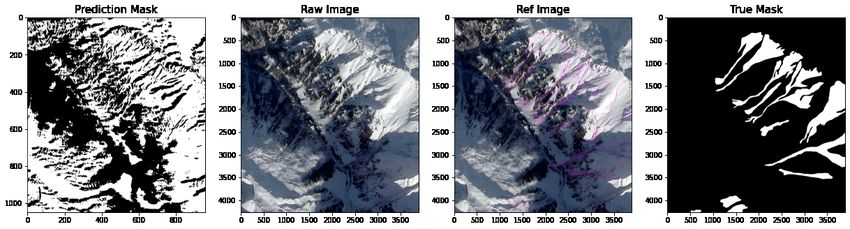
Different model complexities require a finesse to balance feature retention, improve prediction accuracy and reduce
computational cost [22].
    We start by comparing a fully connected CNN with a 1D convolution and a fully connected CNN with a 2D
convolution. In addition, both CNN architectures include additional pooling and normalization layers to reduce
output data size and retain the most representative features [20, p. 335].
    Next, we compare deeply connected CNNs which ideally retain more feature maps and improve prediction. VGG16
is a deeply connected CNN that uses small filters of convolution along the depth of an RGB image. However, adding
more layers to a deeply connected CNN such as VGG16 has limitations. First, vanishing gradient results in model
overfitting [23]. Next, densely connected models require substantial memory during training [20, p. 330]. Two clever
solutions arise: residual networks, which use skip connections between layers to prevent vanishing gradients and
inception networks which are sparsely connected. We compare a popular residual network model ResNet50 and a
combined inception residual network IRNv2 [18] [19]. All of the deeply connected networks are trained on images
dissimilar to the images of avalanches, however, their feature maps cover huge portions of image data. Using available
architectures, we can reduce required computation time of the model and supplement feature detection after training.
    For all model architectures, we use optimizers Adam and RMSProp and a base learning rate of 0.001. In addition,
we use a binary crossentropy loss function with a logit predictor function for numerical stability [24]. At prediction
time, this loss function produces a binary set of predictions for avalanche classification. With these predictions, we
can enhance edge features and threshold values to produce a more precise shape prediction.
    A fully connected architecture with multiple convolution operations and activation applied is computationally
expensive. At model training, we use data generators to randomize the selection of training data batches and free
RAM for future batch training. In addition, we use a distributed TPU cluster on Google Colaboratory with 8 cores,
which substantially reduces training time. TPU availability is limited and at times would require processing with
the CPU, which is impractical for producing time-restricted predictions of avalanche occurrence. Consequently, we
examine potential techniques for improved prediction precision with preliminary analysis of sunny and shady images
for which optimal CNN models have imprecise prediction outcomes. We explore preliminary RGB analysis for future
prediction model improvement.

3.2    Data Preparation
    In addition to the CNN’s architecture, data preparation methods greatly influence computational cost. The data
is sampled from three sets of images including the original unedited image, a reference image outlining the avalanche
with a polygon and a segmented mask of the outline. Each set contains sixty images in jpg format. The folder
images contains original raw satellite images. The set references are images which contain a manually drawn
outline which approximate the true avalanche area. The reference outline is used to threshold pixel values within
the avalanche polygon to 255 (white) and outside to 0 (black). The resulting segmentation is the set of images in
the masks file. Since we are interested in a binary classification problem then we want to create a set of predictor
variables that explains avalanche features to which we fit a binary response variable. We choose to extract data from
the raw images by separating the image into sections or ’windows’ to analyze features. A natural response variable
then is corresponding data in the segmented mask.
    In general, the data are prepared to create multidimensional arrays out of sections of the image or ’windows’
to analyze. Each image t for 0 ≤ t < 60 has height H for 0 ≤ i < H and width W where 0 ≤ j < W with
depth d for 0 ≤ k < d ∈ {1, 3}. We sample data as scalar values where the value p of image t at the ith row, jth
column and kth depth is specified by the function V (i, j, k, t). Each value p uniquely determined by V (i, j, k, t) is
an integer in the range [0, 255]. For a single image t, we separate the data into windows, which are 2−dimensional
arrays with dimensions determined by a selected height h and width w where 0 ≤ i < h < H, 0 ≤ j < w < W. We
sample N windows from t such that the window 0 ≤ n < N has pixel value at row i, column j determined by the
function X(i, j, k, t, n). For each value X(i, j, k, t, n), we sample from mask m the value at the center of the window in
X(i, j, k, m, n), using a buffer defined by b = (h − 1)/2, we determine the corresponding value in m with the function
Y (i + b, j + b, k, t, m).
    We further prepare the masks by performing a binary threshold for values, such that if the mask value 127 ≤
V (i, j, k, m) ≤ 255 then V (i, j, k, m) = 1 otherwise V (i, j, k, m) = 0. For all N windows sampled from t by the
function X(i, j, k, t, n) we have a corresponding binary value determined by Y (i + b, j + b, k, t, m). Let X be all
possible values determined by X(i, j, k, t, n) and let y be all possible values from Y (i + b, j + b, k, t, m).
    The windows in X are the inputs to the model architecture where a batch of windows are selected from X to
be the input nodes of the CNN and y are the response variables to which we fit X. Thus we can tune the features
extracted by the CNN by comparing data generation parameters. For windows we select a size where h = w and
h, w ∈ 17, 33, and image depth d ∈ {1, 3}. From size and depth we have the input shape for the CNN architecture

                                                            2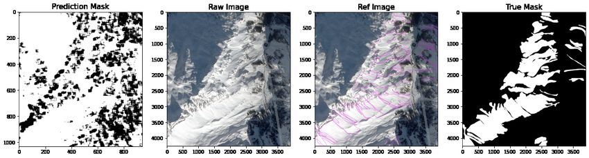
such that input = (h, w, d). Avalanche occurrence may also be influenced by sunlight and shady slopes, implying
color features are important to retain for model training ??. Thus, we compare a CNN with input shape (17, 17, 1)
and a CNN with shape (17, 17, 3) to compare feature detection of models trained with d = 1 for grayscale and d = 3
for red, green and blue channel (RGB) images. The assumption is that larger window sizes will retain edge features
important for avalanche detection [20]. Improving feature detection, we increase the CNN input shape to (33, 33, 3)
and also utilize pre-trained models which cover extensive feature data. Remaining models have input shape (33, 33, 3)
with the exception of IRNv2, which requires input shape (76, 76, 3) [19].
A limiting factor to retaining features is the computational cost of increasing dimensions during data generation.
The complex shape of an avalanche polygon suggests data sampling which iterates per pixel along the height and
width of an image [20, p. 334]. This is an overlapping data sampling method which has redundant data, but can
detect where a particular edge appears [20, p. 334]. However, sampling N windows along each row and column of the
image height and width and along its depth 0 < k ≤ d requires substantial memory use. With high-RAM settings
we have 35GB= 3.5 × 1010 bytes available. Applying an overlapping sampling method without padding to an image
t with dimensions (H, W, d) we can generate N total windows with the function X(i, j, k, m, n) such that N is given
by
Xd XH XW
N= k j i.
k=1 j=1 i=1
Further, a window size of (h, w) would retain m pixel values given by
h
X w
X
m= j i
j=1 i=1
so that the order of the overlapping scheme is given by O(m · N ).
For instance, an image t with dimensions (H, W, d) = (4256, 3694, 3) would generate
3
X 4256
X 3694 X
N= k j i = 370943582819040 ≈ 37 × 1013
k=1 j=1 i=1
Then, if (h, w) = (33, 33), the number of values retained per window is
33
X 33
X
m= j i = 314721.
j=1 i=1
Then the total memory required is approximately 12 × 1019 bytes, which is almost double the amount of available
memory. Instead, we utilize a scaling method by applying a kernel which approximates a Gaussian pyramid [25].
This kernel is given by
1 4 6 4 1
4 16 24 16 4
1
6
24 36 24 6
16
4
16 24 16 4
1 4 6 4 1
The Gaussian pyramid kernel is a useful solution to memory limitations, since each scaling reduces the height H
and width W of an image t by half [3]. A caveat is the loss of resolution and important data specific to the avalanche
edge features (Figure 1).
Instead, we take advantage of model architectures that use larger input shape dimensions and are trained on an
extensive set of imaging data. We use models VGG16, RN50 and IRNv2 that enhance a CNN base model’s feature
detection with RGB and precise edge features.
3.3 Prediction Architecture
Initially, we perform prediction with a more complex architecture using a CNN with Xgboost head architecture.
We use the most optimal architecture and feature maps for this CNN which were provided by the sponsors. With
a binary crossentropy loss function we apply an extreme gradient boosted decision tree on CNN predictions. Since
3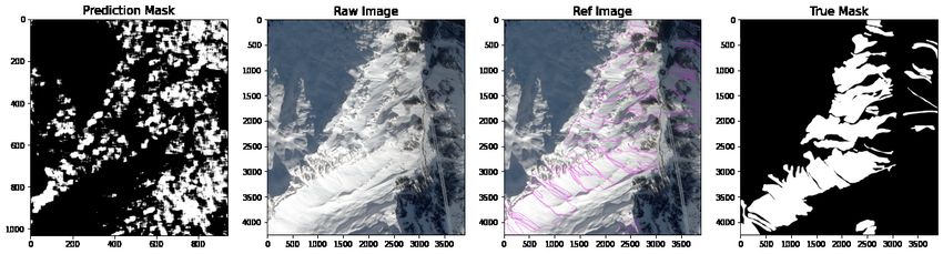
Figure 1: Gaussian kernel applied twice to an image. The image is reduced by half of its previous size after each
matrix multiplication and reduction, reducing distinct avalanche edge features.

the models are trained with a small learning rate of 0.001, the CNN predictions tend towards maximizing the
difference between the learning rate and the true value. An approach to improve this outcome is to use an extreme
gradient boosted decision tree method called Xgboost to fit on the CNN model’s predictions. The method Xgboost
minimizes CNN prediction outputs, reducing overfit predictions This produces prediction data with a distribution
less concentrated towards the true classes.
    The data for model predictions are prepared with the same method that training data is, resulting in another
bottleneck. Instead, we compare prediction architecture by using enhanced features created by CNN predictions,
apply an additional prediction and threshold the image using maximum feature values.

4     Results
4.1    Training
    The training and validation accuracy plots of the 2D CNN with shape (17, 17, 1) versus the 2D CNN with input
shape (17, 17, 3) show a difference in model overfitting (Figure 2). The grayscale data with one channel plateaus
immediately whereas the RGB data does not plateau but a higher validation accuracy suggests an overfit model.
Looking at the 2D CNN with a larger input size (33, 33, 3) between the first two epochs we see more curvature but
another overfit model with higher validation accuracy. The VGG16 architecture is the first to achieve a more optimal
bias-variance trade-off but with an close validation accuracy. The RN50 architecture has inconsistent validation
accuracy. The IRNv2 model’s training and validation accuracy are more smooth with a distinct separation at the
last training epoch.

                                                         4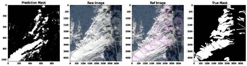
Figure 2: Comparison of model training accuracy versus validation accuracy.

    Comparing model times given in Table 1. the 2D CNN with input shape (33, 33, 3) took approximately 1 minute
to train and also consumes the most RAM out of all model input types. The 2D CNN with shape (17, 17, 3) only
required 44 seconds to train. IRNv2 and RN50 architectures require substantial training time at 22 and 52 minutes.

                  CNN(17,17,1)     CNN(17,17,3)    CNN(33,33,3)    VGG-16      RN-50      IRNv2
                    15.77s           44.46s          67.32s        2m 48s     22m 50s    22m 52s

                                  Table 1: Comparison of model training time.

   A comparison of prediction loss and training accuracy show that the 2D CNN with input shape (17, 17, 1) had
prediction accuracy of 0.922 and prediction loss of 1.02, suggesting overfit data and a poor model for prediction
analysis. The remaining CNN models still achieved at least 0.874 prediction accuracy. (Table 2).

                                                        5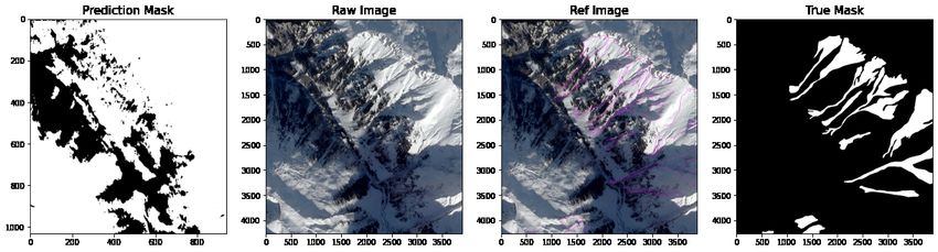
Model            Prediction Loss       Prediction Accuracy
                           CNN (17, 17, 1)           1.02                    0.922
                           CNN (17, 17, 3)          0.367                    0.874
                           CNN (33, 33, 3)          0.367                    0.876
                          VGG16 (33, 33, 3)         0.310                    0.901
                           RN50 (33, 33, 3)         0.310                    0.901
                          IRNv2 (76, 76, 3)         0.310                    0.901

                            Table 2: Prediction loss and accuracy compared for models.

Figure 3: Evaluating training loss and test accuracy for models: (A) CNN (17, 17, 1) (B) CNN (17, 17, 3) (C) (33, 33, 3)
(D) VGG16 (33, 33, 3) (E) RN50 (33, 33, 3) (F) IRNv2 (76, 76, 3).

                                              Figure 4: Prediction losses

                                                           6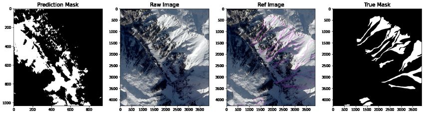
4.2 Prediction
4.2.1 CNN with Xgboost Predictions
Predictions on an image using both models required extensive computational time which resulted in runtime
disconnection from Google Colaboratory. As an alternative, using four separate tiles from the image we were able to
produce predictions but the predictions were sparse (Figure 5).
Figure 5: Predictions using tiles to reduce time of computation with sparse outcomes. Compared to mask, reference
and original image.
4.2.2 CNN Predictions
As an alternative to the computationally ineffective CNN with Xgboost model, we used a CNN model prediction
to enhance features in an image. A single prediction on a model transformed the original image to create enhanced
features where possible features include the gradients of the mountain as well as avalanche edges. Since the gradients
include features that we are not interested in classifying we segmented the feature enhanced image. Following, an
additional prediction was made with the same CNN model used for feature enhancement. This was applied for all 2D
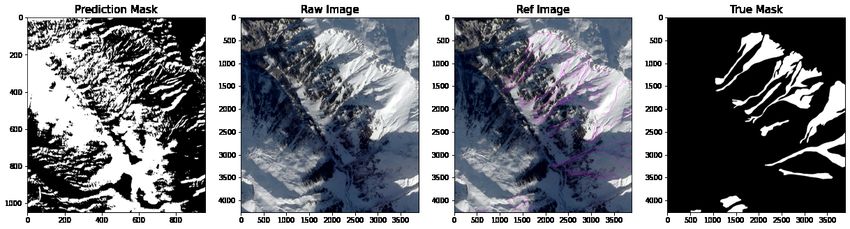
CNN models and the VGG16 architecture. The comparison in Figure 6 shows the CNN (17, 17, 3), CNN (33, 33, 3),
VGG16 and RN50 predictions on the left versus the original, reference and mask image. After making predictions
on a column in the image, a max argument function was used to mark indices in an empty prediction mask with
binary values. We can see concentrated predictions around the gradients of the mountain but with significant noise
to suggest imprecise shape prediction.
Following an initial prediction, we apply a Canny edge detector to the first prediction output. This detects
significant edges in the first prediction set for which we can see shared edges between the edge-enhanced prediction
image and edge-enhanced reference image (Figure 7).
Since there is substantial noise in the first prediction set, we apply an additional prediction operation to the
edge-enhanced prediction. The second prediction output shows a narrowing of the prediction towards the avalanche
polygon in the mask. Similarly to the first prediction, we compare four model predictions from CNN (17, 17, 3), CNN
(33, 33, 3), VGG16 and RN50 against the original, reference and mask image (Figure 8).
7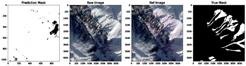
Figure 6: Comparison of model predictions for single CNN prediction using a max value filter and binary threshold
comparing prediction, original, reference and mask. From top to bottom: CNN (17, 17, 3), CNN (33, 33, 3), VGG16
and RN50.

                                                       8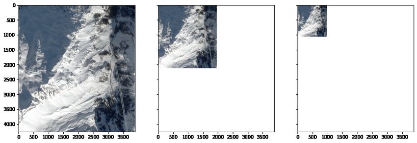
Figure 7: Comparison of Canny edge detection from first CNN predictions on left against reference edges, from top
to bottom: CNN (17, 17, 3), CNN (33, 33, 3), VGG16 and RN50.

                                                       9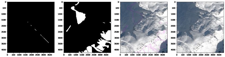
Figure 8: Comparison of model predictions for second CNN prediction made on edge enhanced images using a max
value filter and binary threshold comparing prediction, original, reference and mask. From top to bottom: CNN
(17, 17, 3), CNN (33, 33, 3), VGG16 and RN50.

                                                     10
Figure 9: Comparison of Canny edge detection from second CNN predictions on left against reference edges, from
top to bottom: CNN (17, 17, 3), CNN (33, 33, 3), VGG16 and RN50.
114.3 RGB Analysis
Figure 10: Comparison of histogram results of four sunny (left column) versus four shady (right column) images with
the full RGB depth analyzed. Initial observation implies concentration of pixel values in [100, 150] for shady images
and [200, 250] for sunny images with the exception of index 33 and index 12.
From the set of sixty images four images are classified as sunny and four images are classified as shady. In Figure
10 we compare the RGB histograms of sunny and shady images. From initial analysis we can see three images in
the sunny set with local maximums concentrated near larger pixel values in the range [200, 255]. With the exception
of index 12 which has two local maximums in [200, 255] and [100, 150]. The shady set of images also shows a local
12maximum but with a range less than the sunny images near [100, 150]. A similar result to the sunny images occurs
with index 33 which has a concentration of pixel values near [200, 255]. The three shady images which have pixel
values close to [100, 150] also have a distinct separation of the blue, green and red histograms while the sunny images
have RGB histograms that are almost overlapping. In addition, the shady images have higher hue and saturation
peaks than the sunny images.
5 Discussion
The results from model training suggest that models with higher input dimensions have an optimal bias variance
trade-off. From the model training plots we see that the CNN with input shape (17, 17, 1) immediately overfit when
its validation accuracy plateaued close to the first epoch out of five epochs. This suggests that the variability in an
image with small window size and grayscale depth does not retain edge features for avalanche detection but may
instead retain contrast features of a grayscale image. The next level of model complexity for the same window size of
17 but with RGB depth showed improvement in training and validation curve shape. The curvature is not enough to
prevent an overfit model as we see the validation accuracy is greater than the training accuracy. From initial CNN
(17, 17, 1) and CNN (17, 17, 3) analysis, we infer that RGB data should be retained.
We assumed that larger window size would improve model performance which is true for preexisting architectures
VGG16, RN50 and IRNv2 but is not the case for CNN (33, 33, 3). While a larger window size would retain more
features, recall that a required Gaussian pyramid scaling reduced some of the original features in the RGB image. This
is confirmed when looking at the CNN (33, 33, 3) model plot which also has a higher validation accuracy suggesting
an overfit model. Thus, the models which are already trained and have extensive feature information had the best
bias-variance tradeoff. This suggests that a complex or custom architecture is not necessary to improve the model’s
accuracy. Instead, building on an already existing architecture to enhance features that are important for polygon
detection is more important and also feasible in terms of time and computation. Looking at the model accuracy
plots again, we can see that the model with the best bias-variance tradeoff is the IRNv2 model. This may be the case
since IRNv2 uses very small convolution kernel shape which may detect small edge occurrences that are unique to
the avalanche polygon. The results from training analysis also suggest that edge detection concerns small gradients
in the image versus edges created by image contrast. In addition, the potential contrast created by RGB data may
be correlated to variable data from the image hue and saturation.
Performing predictions with the model architectures CNN (17, 17, 3), CNN (33, 33, 3), VGG16 and RN50 show
that initial predictions produce significant noise. Using Canny edge detection we were able to enhance features
related to the gradients of the mountain, the avalanche edge and other natural elements on the mountain. A second
prediction on these edge-enhanced images greatly improved the binary output and narrowed the region of prediction.
While a final edge enhancement observations suggest that VGG16 edges are comparable with the reference edges.
Since VGG16 is densely connected and trained on the full image depth of many images, this suggests again the
importance of RGB data.
The results from training and prediction analysis lead to the desire to create a model that incorporates RGB
complexity at training time but has precise prediction accuracy. Looking at the preliminary RGB histogram analysis,
we can see a potential difference between hue and saturation concentration near pixel values. Sunny images have
local maximums at a higher pixel value range with smaller intensities where RGB curves overlap. In contrast, shady
images have local maximums at a lower pixel value range with higher intensities and distinct separations between
RGB channels. This suggests in addition to avalanche binary classification a category of sunny or not sunny is also
important.
6 Conclusion
With a base model architecture already in place, precise avalanche polygon prediction requires further refinement
of previously inferred important features. A higher resolution image with more RGB features for model training
would be suggested. Still restricted by the available memory, potential solutions would use Principal Component
Analysis to reduce dimensionality, where preliminary analysis shows 9 transformed features account for 99% of the
feature variation. In addition, the importance of edge features during prediction analysis suggests creating a best
set of corner coordinates from prediction edges. Since the prediction images have substantial noise and additional
edges then a minimizing model objective would be appropriate. A return to the Xgboost model may be suitable to
fit extracted prediction coordinates with avalanche polygon coordinates in the mask. Following, available numerical
analysis techniques like cubic spline interpolation may be suggested to refine the polygon area and reduce initial
prediction noise by bounding outputs with a polygon region.
137 Required Files
• Input files: images, masks and reference images which are available in the ’data’ folder
• ultimate_notebook.ipynb
• Google Colaboratory runtime: go to Runtime > Change runtime type and select ’TPU’ and ’High-Ram’.
Note: the separate models are loaded to avoid restarting the TPU which may interrupt execution of the
notebook.
14References
[1] Tensor:
https://mathworld.wolfram.com/Tensor.html
[2] CategoricalCrossentropy
https://www.tensorflow.org/apid ocs/python/tf /keras/losses/CategoricalCrossentropy
[3] Image Pyramids:
https://docs.opencv.org/2.4/doc/tutorials/imgproc/pyramids/pyramids.html
[4] PCA Decomposition:
https://scikit-learn.org/stable/modules/generated/sklearn.decomposition.PCA.html
[5] Jake VanderPlas Python Data Science Handbook Essential Tools for Working with Data, O’Reilly Media, Novem-
ber 2016
https://jakevdp.github.io/PythonDataScienceHandbook/05.09-principal-component-analysis.html
[6] Karen Simonyan, Andrew Zisserman Very Deep Convolutional Neural Networks for Large-Scale Image Recognition
https://arxiv.org/pdf/1609.04747.pdf
[7] StandardScaler:
https://scikit-learn.org/stable/modules/generated/sklearn.preprocessing. StandardScaler.html
[8] Michael E. Tipping and Christopher M. Bishop, Mixtures of Probabilistic Principal Component Analysers
http://www.miketipping.com/papers/met-mppca.pdf
[9] Sequential:
https://keras.io/getting-started/sequential-model-guid
[10] Sebastian Ruder, An overview of gradient descent optimization algorithms
https://arxiv.org/pdf/1609.04747.pdf
[11] Diederik P. Kingma,Jimmy Lei Ba, Adam: a Method for Stochastic Optimization
https://arxiv.org/pdf/1412.6980v8.pdf
[12] Christian Szegey, Alexander Toshev, and Dumitru Erhan, Deep Neural Networks for Object Detection, from
Advances in Neural Information Processing Systems 26,
https://papers.nips.cc/paper/5207-deep-neural-networks-for-object-detection.pdf
[13] Matthew D. Zeiler, Rob Fergus, Visualizing and Understanding Convolutional Networks
https://arxiv.org/pdf/1311.2901.pdf
[14] Mesay Belete Bejiga,Abdallah Zeggada,Abdelhamid Nouffidj and Farid Melgani, A Convolutional Neural Net-
work Approach for Assisting Avalanche Search and Rescue Operations with UAV Imagery
https://www.mdpi.com/2072-4292/9/2/100
[15] Anne Bonner The Complete Beginner’s Guide to Deep Learning: Convolutional Neural Networks and Image
Classification Conquer the basics of CNNs and image classification in mere minutes
https://towardsdatascience.com/wtf-is-image-classification-8e78a8235acb
[16] Davi Frossard VGG in TensorFlow Model and pre-trained parameters for VGG16 in TensorFlow
https://www.cs.toronto.edu/ frossard/post/vgg16/
[17] Vishal Morde XGBoost Algorithm: Long May She Reign! The new queen of Machine Learning algorithms taking
over the world. . .
https://towardsdatascience.com/
https-medium-com-vishalmorde-xgboost-algorithm-long-she-may-rein-edd9f99be63d
[18] Priya Dwivedi Understanding and Coding a ResNet in Keras Doing cool things with data!
https://towardsdatascience.com/understanding-and-coding-a-resnet-in-keras-446d7ff84d33
[19] Bharath Raj A Simple Guide to the Versions of the Inception Network
https://towardsdatascience.com/a-simple-guide-to-the-versions-of-the-inception-network-7fc52b863202
15[20] Ian Goodfellow, Yoshua Bengio and Aaron Courville Deep Learning, MIT Press, 2016,
http://www.deeplearningbook.org
[21] Francois Challet Deep Learning with Python, Manning Publications Co., 2018,
[22] Simone Bianco, Remi Cadene, Luigi Celona and Paolo Napoletano, Benchmark Analysis of Representative Deep
Neural Network Architectures
https://arxiv.org/pdf/1810.00736.pdf
[23] Roger Grosse Lecture 15: Exploding and Vanishing Gradients
http://www.cs.toronto.edu/ rgrosse/courses/ csc3212 017/readings/
L15%20Exploding%20and%20V anishing%20Gradients.pdf
[24] BinaryCrossentropy
https://www.tensorflow.org/apid ocs/python/tf /keras/losses/BinaryCrossentropy
[25] Matthew Aubery, Wayne Luck Binomial Filters
http://citeseerx.ist.psu.edu/viewdoc/download?doi=10.1.1.43.7611rep=rep1type=pdf
16You can also read