Learning to parse images of articulated bodies
←
→
Page content transcription
If your browser does not render page correctly, please read the page content below
Learning to parse images of articulated bodies

                                          Deva Ramanan
                              Toyota Technological Institute at Chicago
                                        Chicago, IL 60637
                                     ramanan@tti-c.org

                                              Abstract

         We consider the machine vision task of pose estimation from static images, specif-
         ically for the case of articulated objects. This problem is hard because of the large
         number of degrees of freedom to be estimated. Following a established line of
         research, pose estimation is framed as inference in a probabilistic model. In our
         experience however, the success of many approaches often lie in the power of the
         features. Our primary contribution is a novel casting of visual inference as an it-
         erative parsing process, where one sequentially learns better and better features
         tuned to a particular image. We show quantitative results for human pose estima-
         tion on a database of over 300 images that suggest our algorithm is competitive
         with or surpasses the state-of-the-art. Since our procedure is quite general (it does
         not rely on face or skin detection), we also use it to estimate the poses of horses
         in the Weizmann database.

1   Introduction
We consider the machine vision task of pose estimation from static images, specifically for the case
of articulated objects. This problem is hard because of the large number of degrees of freedom to
be estimated. Following a established line of research, pose estimation is framed as inference in a
probabilistic model. Most approaches tend to focus on algorithms for inference, but in our expe-
rience, the low-level image features often dictate success. When reliable features can be extracted
(through say, background subtraction or skin detection), approaches tend to do well. This depen-
dence on features tends to be under-emphasized in the literature – one does not want to appear to
suffer from “feature-itis”. In contrast, we embrace it. Our primary contribution is a novel casting
of visual inference as an iterative parsing process, where one sequentially learns better and better
features tuned to a particular image. Since our approach is fairly general (we do not use any skin or
face detectors), we also apply it to estimate horse poses from the Weizmann dataset [1].
Another practical difficulty, specifically with pose estimation, is that of reporting results. It is com-
mon for an algorithm to return a set of poses, and the correct one is manually selected. This is
because the posterior of body poses is often multimodal, a single MAP/mode estimate won’t sum-
marize it. Inspired by the language community, we propose a perplexity-based measure for evalua-
tion. We calculate the probability of observing the actual pose under the distribution returned by our
algorithm. With such an evaluation procedure, we can quantifiable demonstrate that our approach
improves the state-of-the-art.
Related Work: Human pose estimation is often approached in a video setting, within the context of
tracking. Space does not allow for a proper review. Approaches date back to the model-based tech-
niques of Hogg [5] and ORourke and Badler [11]. Recent focus in the area has expanded to single-
image pose estimation, because such algorithms are likely useful for tracker (re)-initializiation. Top-
down approaches match an image to a set of templates spanning a range of body poses [17, 9, 19].
Bottom-up approaches first detect body parts in an image, and then reason about their geometric
relationship. This search over body part locations can be algorithmically complex, and sampling-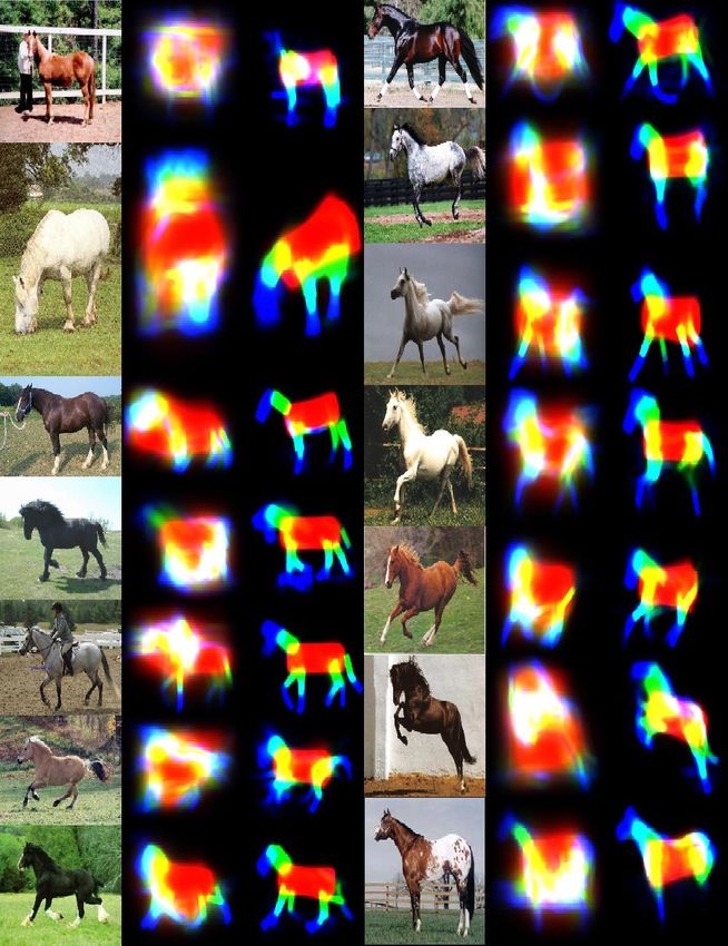
Figure 1: The curse of edges? Edges are attractive because of their invariance – they fire on dark
objects in light backgrounds and vice-versa. But without a region model, it can be hard to separate
the figure from the background. We describe an iterative algorithm for pose estimation that learns
a region model for each body part and for the background. Our algorithm is initialized by the edge
maps shown; we show results for these two images in Fig.7 and Fig.8.
based schemes are common [8, 4, 6, 18]. Instead, we rely on a version of the tree-structured model
from [3, 15], which allows for efficient inference. Specifically, we use the conditional random field
(CRF) notion of deformable matching from [13]. Bottom-up approaches seem to require good part
detectors. But building accurate detectors is hard because of nuisance factors like illumination and
clothing. One approach is to use people-specific cues, such as face/skin/hair detection[8, 4, 20].
We describe an approach that iteratively learns good part models for a particular image, while si-
multaneously estimating the pose of the articulated object in that image. Our approach is related
to those that simultaneously estimate pose and segment an image [10, 14, 2, 7], since we learn
low-level segmentation cues to build part-specific region models. However, we compute no explicit
segmentation.
1.1 Overview
Assume we are given an image of a person, who happens to be a soccer player wearing a white shirt
on a green playing field (Fig. 2). We want to estimate the figure’s pose. Since we do not know the
appearance of the figure or the background, we must use a feature invariant to appearance (Fig.1).
We match an edge-based deformable model to the image to obtain (soft) estimates of body part posi-
tions. In general, we expect these estimates to be poor because the model can be distracted by edges
in the background (e.g., the hallunicated leg and the missed arm in Fig. 2). The algorithm uses the
estimated body part positions to build a rough region model for each body part and the background –
it might learn that the torso is white-ish and the background is green-ish. The algorithm then builds
a region-based deformable model that looks for white torsos. Soft estimates of body position from
the new model are then used to build new region models, and the process is repeated.
As one might suspect, such an iterative procedure is quite sensitive to its starting point – the edge-
based deformable model used for initialization and the region-based deformable model used in the
first iteration prove crucial. As the iterative procedure is fairly straightforward (Fig.3), most of this
paper deals with smart ways of building the deformable models.
2 Edge-based deformable model
Our edge-based deformable model is an extension of the one proposed in [13]. The basic proba-
bilistic model is a tree-structured conditional random field (CRF). Let the location of each part li
be parameterized by image position and orientation [xi , yi , θi ]. We will assume parts are oriented
patches of fixed size, where (xi , yi ) is the location of the top of the patch. We denote the configura-
tion of a K part model as L = (l1 . . . lK ).
We can write the deformable model as a log-linear model
X X
P(L|I) ∝ exp ψ(li − lj ) + φ(li ) (1)
i,j∈E i
Ψ(li − lj ) corresponds to a spatial prior on the relative arrangement of part i and j. For efficient
inference, we assume the edge structure E is a tree; each part is connected to at most one parent.
Unlike most approaches that assume gaussian shape priors [13, 3], we parameterize our shape model
initial parse

                                                                                                         missing arm

                                                                                                                           torso              head

                                                                                                   hallucinated leg

                                                                                                                          ru−arm            ll−leg

Figure 2: We build a deformable pose model based on edges. Given an image I, we use a edge-
based deformable model (middle) to compute body part locations P(L|I). This defines an initial
parse of the image into several body part regions right. It is easy to hallucinate extra arms or legs
in the negatives spaces between actual body parts (the extra leg). When a body part is surrounded
by clutter (the right arm), it is hard to localize. Intuitively, both problems can be solved with low-
level segmentation cues. The green region in between the legs is a poor leg candidate because of
figure/ground cues – it groups better with the background grass. Also, we can find left/right limb
pairs by appealing to symmetry – if one limb is visible, we can build a model of its appearance, and
use it to find the other one. We operationalize both these notions by our iterative parsing procedure
in Fig.3.
                                                                                                         re−parse with
                                                                                                          additional
                                                                                                           features

                                                             learn                                                                               arm found
                                                             part−
                                                            specific
                                                             fg/bg                                                       iter1
                           torso            head            models          torso           head

                     weak arm response

                                                                                                                                         suppress
                                                                                                                                         false leg
 initial posterior
   from edges                                                                                                                                iter3
                                             hallucinated
                                                  leg
                      lower l/r arms     lower l/r legs                lower l/r arms   lower l/r legs                   iter2

Figure 3: Our iterative parsing procedure. We define a parse to be a soft labeling of pixels into
a region type (bg,torso,left lower arm, etc.). We use the initial parse from Fig.2 to build a region
model for each part. We learn foreground/background color histogram models. To exploit symmetry
in appearance, we learn a single color model for left/right limb pairs. We then label each pixel using
the color model (middle right). We then use these masks as features for a deformable model that
re-computes P(L|I). This in-turn defines a new parse, and the procedure is repeated.

with discrete binning (Fig.2).
                                                          ψ(li − li ) =αiT bin(li − lj )                                                              (2)

Doing so allows us to capture more intricate distributions, at the cost of having more parameters
to fit. We write bin(·) for the vectorized count of spatial and angular histogram bins (a vector of
all zeros with a single one for the occupied bin). Here αi is a model parameter that favors certain
(relative) spatial and angular bins for part i with respect to its parent.
Φ(li ) corresponds to the local image evidence for a part, which we define as
                                                                 φ(li ) =βiT fi (I(li ))                                                              (3)

We write fi (I(li )) for feature vector extracted from the oriented image patch at location li . In
general, fi () might be part-specific; it could return a binary vector of skin pixels for the the head. In
our case, fie returns a binary vector of edges for all parts. We can visualize βi in Fig.6.
final parse sample poses
best pose
Figure 4: The result of our procedure.
Given P(L|I) from the final iteration,
torso head we obtain a clean parse for the image.
We can also compute L̂M AP (the most
likely pose), and can sample directly
input
from P(L|I).
ru−arm ll−leg
Figure 5: We record the spatial configuration of an arm given the torso by placing a
grid on the torso, and noting which bin the arm falls into. We center the grid at the
average location of arm in the training data. We likewise bin the angular orientations
to define a spatial distribution of arms given torsos.
Inference: The basic machinery we use for inference is message-passing (the sum-product algo-
rithm). Since E is a tree, we first pass “upstream” messages from part i to its parent j
We compute the message from part i to j as
X
mi (lj ) ∝ ψ(li − lj )ai (li ) (4)
lj
Y
ai (li ) ∝ φ(li ) mk (li ) (5)
k∈kidsi
Message passing can be performed exhaustively and efficiently with convolutions. If we temporarily
ignore orientation and think of li = (xi , yi ), we can represent messages as 2D images. The image ai
is obtained by multiplying together response images from the children of part i and from the imaging
model φ(li ). φ(li ) can be computed by convolving the edge image with the filter βi . mi (lj ) can be
computed by convolving ai with a spatial filter extending over the bins from Fig.2 (with coefficients
equal to αi ). At the root, the image ai is the true conditional marginal P(li |I). When li is 3D, we
perform 3D convolutions. We assume αi is separable so convolutions can be performed separately
in each dimension. This means that in practice, computing φ(li ) is the computational bottleneck,
since that requires convolving the edge image repeatedly with rotated versions of filter βi .
Starting from the root, we can pass messages downstream from part j to part i (again with convolu-
tions)
X
P(li |I) ∝ ai (li ) ψ(li − lj )P(lj |I) (6)
lj
For numerical stability, we normalize images to 1 as they are computed. By keeping track of the
normalization constants, we can also compute the partition function (which is needed for computing
the evaluation score in Sec. 5).
Learning: We learn the filters αi and βi by CRF parameter estimation, as in [13]. We label training
images with body part locations L, and find the filters that maximize P(L|I) for the training set.
This objective function is convex and so we tried various optimization packages, but found simple
stochastic gradient ascent to work well. We define the model learned from the edge feature map fie
as Θe = {αie , βie }.
3 Building a region model
One can use the marginals (for say, the head) to define a soft labeling for the image into head/non-
head pixels. One can do this by repeatedly sampling a head location (according to P(li |I)) and then
rendering a head at the given location and orientation. Let the rendered appearance for part i be animage patch si ; we use a simple rectangular mask. In the limit of infinite samples, one will obtain
an image
X
pi (x, y) = P(xi , yi , θi |I)sθi i (x − xi , y − yi ) (7)
xi ,yi ,θi
We call such an image a parse for part i (the images on the right from Fig. 2). It is readily computed
by convolving P(li |I) with rotated versions of patch si . Given the parse image pi , we learn a color
histogram model for part i and “its” background.
X
P(f gi (k)) ∝ pi (x, y)δ(im(x, y) = k) (8)
x,y
X
P(bgi (k)) ∝ (1 − pi (x, y))δ(im(x, y) = k) (9)
x,y
We use the part-specific histogram models to label each pixel as foreground or background with a
likelihood ratio test (as shown in Fig.3). To enforce symmetry in appearance, we learn a single color
model for left/right limb pairs.
4 Region-based deformable model
After an initial parse, our algorithm has built an initial region model for each part (and its back-
ground). We use these models to construct binary label images for part i: P(f gi (im)) > P(bgi (im)).
We write the oriented patch features extracted from these label images as fir (for “region”-based).
We want to use these features to help re-estimate the pose in an image – we using training data to
learn how to do so. We learn model parameters for a region-based deformable model Θr by CRF
parameter estimation, as in Sec.2.
When learning Θr from training data, defining fir is tricky – should we use the ground-truth part
locations to learn the color histogram models? Doing so might be unrealistic – it assumes at “run-
time”, the edge-based deformable model will always correctly estimate part locations. Rather, we
run the edge-based model on the training data, and use the resulting parses to learn the color his-
togram models. This better mimics the situation at run-time, when we are faced with a new image
to parse.
When applying the region-based deformable model, we have already computed the edge responses
φe (li ) = βie T f e (I(li )) (to train the region model). With little additional computational cost, we
can add them as an extra feature to the region-based map fir . One might think that the region-
features eliminate the need for edges – once we know that a person is wearing a white shirt in a
green background, why bother with edges? If this was the case, one would learn a zero weight for
the edge feature when learning βir from training data. We learn roughly equal weights for the edge
and region features, indicating both cues are complementary rather than redundant.
Given the parse from the region-based model, we can re-learn a color model for each part and the
background (and re-parse given the new models, and iterate). In our experience, both the parses and
the color models empirically converge after 1-2 iterations (see Fig. 3).
5 Results
We have tested our parsing algorithm on two datasets. Most people datasets are quite small, limited
to tens of images. We have amassed a dataset of 305 images of people in interesting poses (which
will be available on the author’s webpage). It has been collected from previous datasets of sports
figures and personal pictures. To our knowledge, it is the largest labeled dataset available for human
pose recognition. We also have tested our algorithm on the Weizmann dataset of horses [1].
Evalutation: Given an image, our parsing procedure returns a distribution over poses P(L|I). Ide-
ally, we want the true pose to have a high probability, and all other poses to have a low value. Given
a set of T test images each with a labeled ground-truth pose L̂t , we score performance by computing
− T1 t log P(L̂t |It ). This is equivalent to standard measures of perplexity (up to a log scale) [16].
PFigure 6: We visualize the part models for our deformable templates – light areas correspond to pos-
itive βi weights, and dark corresponds to negative. It is crucial to initialize our iterative procedure
with a good edge-based deformable model. Given a collection of training images with labeled body
parts, one could build an edge template for each part by averaging (left) – this is the standard maxi-
mum likelihood (ML) solution. As in [13], we found better results by training βie with a conditional
random field (CRF) model (middle). The CRF edge templates seem to emphasize different features,
such as the contours of the head, lower arms, and lower torso. The first re-parsing from Fig.3 is
also very crucial – we similarly learn region-based part templates βir with a CRF (right). These
templates focus more on region cues rather than edges. These templates appear more sophisticated
than rectangle-based limb detectors [12, 13] – for example, to find upper arms and legs, it seems
important to emphasize the edge facing away from the body.
Log-probability of images given model
Comparison with previous work
Iter 0 Iter 1 Iter2
Previous Iter 0 Iter 1
PeopleAll 62.33 55.60 57.39
USCPeople 55.85 45.77 41.49
HorsesAll 51.81 47.76 45.80
Table 1: Quantitative evaluation. For each image, our parsing procedure returns a distribution of
poses. We evaluate our algorithm by looking at a perplexity-based score [16] – the negative log
probability of the ground truth pose given the estimated distribution, averaged over the test set. On
the left, we look at the large datasets of people and horses (each with 300 images). Iter0 corresponds
to the distribution computed by the edge-based model, while Iter1 and Iter2 show the results after our
iterative parsing with a region-based model. For people, we achieve the best performance after one
iteration of the region-based model. For horses, we do better after two iterations. To compare with
previous approaches, we look at performance on the 20 image dataset from USC [13, 8]. Compared
to [13], our model does better at explaining the ground-truth data.
People: We learned a model from the first 100 training images (and their mirror-flipped versions).
We learn both Θe and Θr from the same training data. We have evaluated results on the 205 re-
maining images. We show sample image in Fig.7. We localize some difficult poses quite well, and
furthermore, the estimated posterior P(L|I) oftentimes reflects actual ambiguity in the data (ie, if
multiple people are present). We quantitatively evaluate results in Table 1. We also compare with a
state-of-the-art algorithm from [13], and show better performance on dataset used in that work.
Horses: We learn a model from the first 20 training images, and test it on the remaining 280 images.
In general, we do quite well. The posterior pose distribution often captures the non-rigid deforma-
tions in the body. This suggests we can use the uncertainty in our deformable matching algorithm
to recover extra information about the object. Looking at the numbers in Table 1, we see that the
parses tend do significantly better at capturing the ground-truth poses. We also see that this dataset
is easier overall than our set of 305 people poses.
Discussion: We have described an iterative parsing approach to pose estimation. Starting with an
edge-based detector, we obtain an initial parse and iteratively build better features with which to
subsequently parse. We hope this approach of learning image-specific features will prove helpful in
other vision tasks.
References
[1] E. Borenstein and S. Ullman. Class-specific, top-down segmentation. In ECCV, 2002.
[2] M. Bray, P. Kohli, and P. Torr. Posecut: simultaneous segmentation and 3d pose estimation of humans
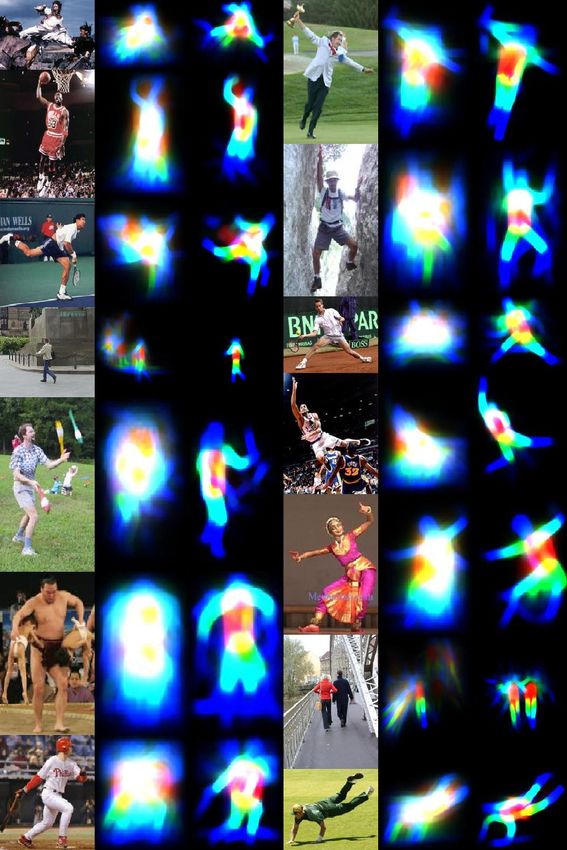
using dynamic graph-cuts. In ECCV, 2006.Figure 7: Sample results. We show the original image, the initial edge-based parse, and the final
region-based parse. We are able to capture some extreme articulations. In many cases the posterior is
ambiguous because the image is (ie, multiple people are present). In particular, it may be surprising
that the pair in the bottom-right both are recognized by the region model – this suggests that the
the iter-region dissimilarity learned by the color histograms is a much stronger than the foreground
similarity. We quantify results in Table 1.
[3] P. F. Felzenszwalb and D. P. Huttenlocher. Pictorial structures for object recognition. Int. J. Computer
Vision, 61(1), January 2005.
[4] M.-H. Y. Gang Hua and Y. Wu. Learning to estimate human pose with data driven belief propagation. In
CVPR, 2005.
[5] D. Hogg. Model based vision: a program to see a walking person. Image and Vision Computing, 1(1):5–
20, 1983.
[6] S. Ioffe and D. Forsyth. Probabilistic methods for finding people. Int. J. Computer Vision, 2001.
[7] M. Kumar, P. Torr, and A. Zisserman. Objcut. In CVPR, 2005.
[8] M. Lee and I. Cohen. Proposal maps driven mcmc for estimating human body pose in static images. In
CVPR, 2004.
[9] G. Mori and J. Malik. Estimating human body configurations using shape context matching. In ECCV,
2002.
[10] G. Mori, X. Ren, A. Efros, and J. Malik. Recovering human body configurations: Combining segmenta-
tion and recognition. In CVPR, 2004.Figure 8: Sample results for horses. Our results tend to be quite good across the entire dataset of 300
images. Even though the horse model is fairly simplistic – a collection of rectangles similar to Fig. 6
– the posterior can capture rich non-rigid deformations of body parts. The Weizmann set of horses
seems to be easier than our people dataset - we quantify this with a perplexity score in Table 1.
[11] J. O’Rourke and N. Badler. Model-based image analysis of human motion using constraint propagation.
IEEE Trans. Pattern Analysis and Machine Intelligence, 2:552–546, 1980.
[12] D. Ramanan, D. Forsyth, and A. Zisserman. Strike a pose: Tracking people by finding stylized poses. In
CVPR, June 2005.
[13] D. Ramanan and C. Sminchisescu. Training deformable models for localization. In CVPR, 2006.
[14] X. Ren, A. C. Berg, and J. Malik. Recovering human body configurations using pairwise constraints
between parts. In ICCV, 2005.
[15] R. Ronfard, C. Schmid, and B. Triggs. Learning to parse picture of people. In ECCV, 2002.
[16] S. Russell and P. Norvig. Artifical Intelligence: A Modern Approach, chapter 23, pages 835–836. Prentice
Hall, 2nd edition edition, 2003.
[17] G. Shakhnarovich, P. Viola, and T. Darrell. Fast pose estimation with parameter-sensitive hashing. In
ICCV, pages 750–757, 2003.
[18] L. Sigal, M. Isard, B. Sigelman, and M. Black. Attractive people: Assembling loose-limbed models using
non-parametric belief propagation. In NIPS, 2003.
[19] J. Sullivan and S. Carlsson. Recognizing and tracking human action. In European Conference on Com-
puter Vision, 2002.
[20] J. Zhang, J. Luo, R. Collins, and Y. Liu. Body localization in still images using hierarchical models and
hybrid search. In CVPR, 2006.You can also read