Smoothed Particle Hydrodynamics for Electrophysiological Modeling: an Alternative to Finite Element Methods
←
→
Page content transcription
If your browser does not render page correctly, please read the page content below
Smoothed Particle Hydrodynamics for
            Electrophysiological Modeling:
       an Alternative to Finite Element Methods

    Èric Lluch1,2(B) , Rubén Doste1 , Sophie Giffard-Roisin3 , Alexandre This2,4 ,
          Maxime Sermesant3 , Oscar Camara1 , Mathieu De Craene2 , and
                                 Hernán G. Morales2
         1
             PhySense, ETIC, Universitat Pompeu Fabra, Barcelona, Catalonia
                          2
                            Medisys, Philips Research, France
                               eric.lluch@philips.com
                        3
                           Université Côte d’Azur, Inria, France
                                  4
                                     Inria Paris, France

        Abstract. Finite element methods (FEM) are generally used in cardiac
        3D-electromechanical modeling. For FEM modeling, a step of a suitable
        mesh construction is required, which is non-trivial and time-consuming
        for complex geometries. A meshless method is proposed to avoid meshing.
        The smoothed particle hydrodynamics (SPH) method was used to solve
        an electrophysiological model on a left ventricle extracted from medical
        imaging straightforwardly, without any need of a complex mesh. The
        proposed method was compared against FEM in the same left-ventricular
        model. Both FEM and SPH methods provide similar solutions of the
        models in terms of depolarization times. Main differences were up to
        10.9% at the apex. Finally, a pathological application of SPH is shown
        on the same ventricular geometry with an added scar on the heart wall.

        Keywords: SPH, Meshless, FEM, Cardiac electrophysiology

1     Introduction
Patient-specific modeling has become an interesting research topic in the car-
diac electrophysiology community because it can help to understand the electri-
cal propagation and its pathologies [2]. FEM is a well-established numerical ap-
proach often used to investigate the electro-mechanics of the human heart [3,13].
The generation of complex meshes is necessary. Meshing is one of the main bot-
tlenecks for the clinical translation of cardiac modeling tools since it is difficult to
have a streamlined and automated pipeline to generate accurate FE simulations
from imaging data [10]. Another non-trivial step of FEM in electro-mechanics is
the coupling between electrophysiology and mechanics when meshes with differ-
ent resolution for both problems are used. It is expected that a way to overcome
these difficulties could be through a meshless approach.
    Various meshless methods have demonstrated the ability to provide a compu-
tational feasible model for cardiac electrophysiology simulations, without burden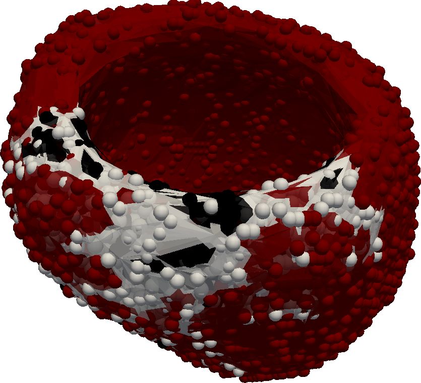
2 Èric Lluch et al
mesh generation [2,5,15]. In this paper, SPH [8] is proposed to numerically solve
the Mitchell-Schaeffer (MS) electrophysiological model [7] on the electrical de-
polarization of the left ventricle. To evaluate the accuracy of this approach, a
comparison with a FEM implementation [6] was conducted. Finally, a scar was
added to the ventricular myocardium to show the potential use of the proposed
meshless approach in a pathological case. The goal is to explore the accuracy,
speed and limitations of SPH with respect to FEM, as a first step towards a
potential full electro-mechanical heart model using a meshless approach.
2 Method
In this section, the electrophysiological model and the SPH discretization scheme
are explained. For further details of the FEM approach, refer to [6].
2.1 Electrophysiological Model
In this paper, the macroscopic biophysical mono-domain model Mitchel-Schaeffer
together with a diffusion term [13] was used to model the cardiac electrophysi-
ology. This model was chosen because it captures the action potential duration
(APD) (Fig. 1), considers fiber orientation in the diffusion term and is only
governed by 6 parameters, which might facilitate a more precise model person-
alization since less parameters need to be fitted to given data.
2
= wv(τ(1−v)
v
∂t v
in
− τout + Iapp
1−w
τopen if v < vgate (1)
∂t w
=2 −w
τclose if v > vgate .
When considering the geometry, a diffusion term div(C∇v) is required to the
first Equation (1) [13]. C ∈ R3,3 is the connectivity tensor defined as
C = (τ ⊗ τ (1 − ar) + Id · ar) · c, (2)
with τ ∈ R3 being the vector corresponding to the fiber orientation, ⊗ the tensor
product, Id ∈ R3,3 the identity matrix, ar ∈ R the anisotropic ratio and c ∈ R
the conductivity coefficient that controls the propagation velocity. ar controls
the conduction velocity in the fiber orientation with respect to the transverse
plane, e.g. in the case ar = 1 , the fiber orientation is not anymore taken into
account, hence reducing the model to the isotropic case.
The parameters τin , τout , τopen , τclose ∈ R control the duration of the four
stages of the APD. The depolarization phase is controlled by w ∈ R and
vgate ∈ R defines at which point the APD starts. Iapp ∈ R corresponds to the
first stimulus of the transmembrane potential v ∈ R.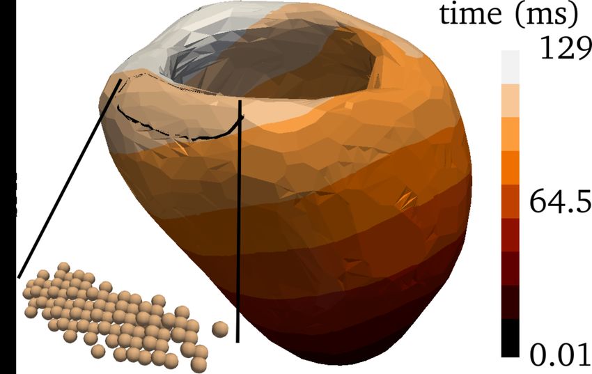
SPH for Electrophysiology               3

Fig. 1: Left: Example of the 4 stages of the cardiac action potential: initiation
(1), plateau (2), decay (3), and recovery (4). Right: Example of an SPH Kernel
for 2D.

2.2   SPH Discretization

SPH is a meshless Lagrangian method, where each solid particle carries its own
properties such as density, conductivity, etc. Given a continuous function f :
R3 → R representing a particle property at the spatial position r, it can be
approximated with a delta Dirac function (3):

                            Z                                Z
   f (r ) = (f ∗ δ)(r ) =        f (r 0 )δ(r − r 0 )dr 0 ≈          f (r 0 )W (r − r 0 , h)dr 0 .   (3)
                            R3                                 R3

Notice that the delta Dirac function was approximated with a kernel function
W (r−r 0 , h), where h ∈ R is the so-called smoothing length (Fig. 1). For Equation
(3) to hold, W must fulfill the following
            Z
                W (r − r 0 , h)dr 0 = 1 and lim W (r − r 0 , h) = δ(r − r 0 ).  (4)
            R3                                    h→0

The integral in (4) is approximated as a finite sum, where the density ρj and
the mass mj are obtained by replacing the infinitesimal volume dr 0 by the finite
volume (5).

                                            f (r 0 )
                                      Z
                   f (r ) = lim                      W (r − r 0 , h)ρ(r 0 )dr 0
                                h→0    R3   ρ(r 0 )
                                N                                                                   (5)
                                X          fj
                            ∝         mj      W (r i − r j , h) = fi ,
                                j=1
                                           ρj

where fi is the approximated value of the function f at the position r, i.e. at
the particle of interest i. Due to the previous formulation (5) the derivative of
the function f in the same position r can be approximated as a derivative of the
kernel function (6)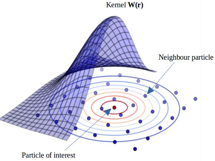
4 Èric Lluch et al
X fj
∇fi = mj ∇W (r i − r j , h). (6)
j
ρj
The electrophysiological model (1) in the SPH formulation reads:
ni
X v j − vi 2
∂t vi = Ci ◦ mj ∇ W (r i − r j , h)
j=1
ρj
wi vi2 (1 − vi ) vi
+ ∇vi div(Ci ) + − + Iapp,i (7)
τin τout
(
1−wi
if vi < vgate
∂t wi = 2 τ−wopen
i
τclose if vi > vgate ,
where ◦ is an element wise multiplication (Hadamard product), ∇2 W ∈ R3,3 is
the Hessian matrix of the kernel including all the Hessian derivatives and
ni ni
X Cj − Ci X vj − vi
∇vi div(Ci ) = mj ∇W (ri − rj , h) · mj ∇W (ri − rj , h),
j=1
ρj j=1
ρj
(8)
where ni is the number of neighbors of the particle pi .
Boundary conditions are difficult to handle in SPH, even when simple bound-
ary conditions such as symmetric surface boundary are required. This is due to
the truncation of the particle neighborhood near a boundary, which results in a
truncation of the integral of equation (5) [4]. Moreover, when it is assumed that
the system connectivity only changes because the particles lose or gain connec-
tivity through a boundary (no-flux), there is no need to place special conditions
on the gradient of the potential function v near the boundary [4, 8]. In other
words, if all the boundaries fulfill the no-flux condition, then the symmetry of
the SPH ensures that the system conserves its flux because the particles inter-
act amongst themselves. On top of this, a corrective smoothed particles method
(CSPM) was implemented to overcome the lack of particles in the boundaries
while enhancing the solution accuracy inside the domain [4]. After applying
CSPM, the discretization scheme has an accuracy of O(h2 ) for interior points
and O(h) for points near or on the boundary, where h is the distance between
particles. The distance depends on the choice of the spatial resolution.
The cubic B-spline kernel (9) was used here since its first derivatives are
positive for neighbor particles close to the particle of interest [4]
1 − 3 q 2 + 3 q 3 for q < 1
0 αd 1 2 3 4
W (x − x , h) = 3 4 (2 − q) for 1 ≤ q < 2 (9)
h
0 elsewhere,
1
where in order to fulfill (4), the coefficient αd = π and q is defined asSPH for Electrophysiology 5
|x − x0 | r
q= = . (10)
h h
Regarding the time integration scheme, a forward explicit Euler method was
used for SPH whose accuracy is O(h), h being the time step. For FEM, the
modified Crank–Nicholson / Adams–Bashforth (MCNAB) was used [13].
3 Experiments
To evaluate the proposed SPH-based electrophysiological model, the same model
was solved with a FEM scheme and results were compared for the electrical
depolarization. An image-based left-ventricular geometry was evaluated in this
work to have a preliminary comparison between the methods. The two methods
are labeled as:
– FEMMS : Mitchell-Schaeffer model discretized with FEM [7].
– SPHMS : Mitchell-Schaeffer model discretized with SPH.
For FEM and SPH approaches, two different resolutions were considered. The
low resolution had 18667 nodes and the high resolution had 51037 nodes for both
approaches. For FEMMS , a tetrahedral mesh was computed from the segmented
left ventricle. For the proposed approach SPHMS , a set of equidistributed points
from the same anatomy was used. Each SPH particle has a density of 1053
kg/m3 , corresponding to reported myocardium density [14]. The mass of each
particle was computed as the product of the density times the volume of the cubic
cell defined between the particle of interest and the neighboring particles. To
understand the impact of key intrinsic parameters of the SPHMS , additional
experiments were conducted for several kernel sizes in these two resolutions.
In order to evaluate the accuracy of these experiments, an analysis of the L2
differences between FEM and SPH activation times, as well as the computational
time, were investigated (Table 1).
For all simulations, myocardial fiber orientation was included in each of the
nodes to achieve a physiological behavior. Fibers were assigned following the
rule-based model angles described by D. Streeter et al. [12]. Regarding the
parameters, an initial electrical impulse Iapp = −580000 mV s was imposed in
a set of points on the apex surface corresponding to 80 mm2 during 4 ms so
that in the first time step with an integration time of dt = 10−4 s an initial
potential of v = −58 mV was obtained. Time variables were τopen = 120 ms,
τclose = 150 ms, τin = 0.3 ms, τout = 6 ms, following [7]. An anisotropic ratio
ar = 0.16 was used.
Moreover, a scar was added in the myocardium of the same left ventricle
to show how SPH handles a pathological example. In particular, the electrical
activation was simulated during one second for both healthy and pathological
scenarios. It was assumed that the heart rate was 75bpm, i.e. the heart period was
0.8 s. Under this assumption, three activation phases were observed within one
simulated second: the depolarization phase, where particles get activated; the6 Èric Lluch et al
repolarization phase, where particles get deactivated; the second depolarization
phase, where particles get activated again. The scar was placed in the septal-
anterior region close to the base. Shape and location of the induced scar are
shown in Fig. 2. The high resolution (51037 particles) model with a kernel size
of 3mm was used for both healthy and pathological simulations. The scar tissue
was applied to 1621 particles while 5891 particles were treated as gray tissue
(tissue near the scar). The rest of the particles were considered as healthy tissue.
Two different pathological experiments with different model parameters were
simulated. In the first pathological simulation, denoted as ’pathological with low
conductivity’, particles in the gray zone and in the scar were modified according
to [1], in such a way that their conductivity coefficient is reduced but not null. In
the second pathological case, denoted as ’pathological with zero conductivity’,
particles in the scar are assumed to have zero conductivity.
Fig. 2: Scar regions in black, Grey zones in grey and healthy zones in red.
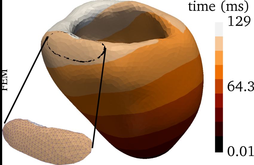
To visualize the discretized domains using both discretization schemes, the
structure of the meshes is shown in Fig. 3. In the case of SPH, a 3D Delaunay
filter from Paraview (Kitware Inc., Clifton Park, USA) was used to enhance
the volume visualization, since unconnected points in 3D do not provide a good
visual 3D representation.
4 Results and Discussion
Results section is structured as follows: first, a sensitivity analysis of the impact
of key intrinsic SPH parameters is presented. Then, a qualitative comparison
against the FEM solution for depolarization is presented. Finally, experiments
to show the SPHMS applicability in a pathological case with a scar are shown.
Depolarization and repolarization phases were compared between healthy and
pathological cases using SPH.
4.1 Sensitivity Analysis
A sensitivity analysis of particle resolution, as well as the kernel size was con-
ducted for SPH and compared against FEM results. Five kernel sizes ranging
from 0.003 to 0.007 m were evaluated. A kernel size < 0.0025 m fails due to
insufficient number of neighbors, while a kernel size > 0.007 m has so manySPH for Electrophysiology 7
neighbors that the computational time was excessive for the potential gain in
accuracy.
Table 1: L2 (R) norm of the difference of depolarization times between SPH and
FEM simulations in the endocardium and computational time (in brackets) of
150 ms with a 4 processor Intel computer for both SPH and FEM.
Number of SPH kernel size
FEM
particles 0.003 0.004 0.005 0.006 0.007
10.294 9.792 9.767 9.500 10.911 –
18667
(37s) (1m13s) (3m13s) (6m43s) (10m43s) (9.92s)
4.258 4.209 4.723 5.103 6.082 –
51037
(4m52s) (11m03s) (21m02s) 38m41s) (57m26s) (27.41s)
Table 1 shows that the L2 error is not linear neither over the kernel size nor over
the resolution. A reduction of the difference between SPH and FEM was observed
when the number of degrees of freedom was incremented for the evaluated kernel
sizes. In terms of computational time, it increases linearly over the kernel size
and faster over the degrees of freedom. The FEM implementation was faster than
the SPH one. A GPU implementation (relatively easy with SPH formulation)
could overcome this disadvantage of the SPH approach [9]. The choice of a kernel
size of 3 mm and a resolution of 51037 particles is a good balance between kernel
size and number of degrees of freedom since the L2 error with respect to FEM
is very small and it was relatively fast to compute. For the rest of the results,
this choice of kernel size and resolution was used.
4.2 Qualitative Comparison
Depolarization times were first qualitatively compared using a discrete colormap
divided by ten isochronous on the ventricle. In all simulations the electrical
activation started from the apex until the septal base. SPHMS and FEMMS show
the same range of depolarization times and a similar activation pattern (Fig. 3).
Moreover, it is observed that all particles in the endocardium get activated after
123 ms. To evaluate the propagation with both approaches, a picture of the
activation times for the same cross section in both approaches is shown in Fig. 3
(middle column). In general, a visual comparison of this figure shows that the
behavior over the whole ventricular volume is similar for both FEM and SPH
methods. The left ventricle endocardium was then mapped into a disk by the
use of Quasi-conformal mapping (QCM) [11] to better visualize differences in all
regions. The mapped results are shown in the bullseye plots of Fig. 3.
To insight into the differences between SPHMS and FEMMS , the absolute differ-
ences between the depolarization times of these two numerical approaches were
computed on the endocardium. These differences were projected on a homeo-
morphic disk as shown in Fig. 4. In this figure, it is observed that the highest8 Èric Lluch et al
Fig. 3: Left: Contour color map of depolarization times for the left ventricle
model. Middle: a longitudinal cross section of the ventricle. Right: projected
endocardium onto a disk for both SPH and FEM simulations.
differences of depolarization times in the endocardium occur near the apex with
a peak difference of 13.5 ms. For most of the domain, the differences are less
than 4 ms as can be seen in the histogram of Fig. 4.
1,500 Septal
Number of Points
Lateral
1,000
Anterior
Posterior
500
0
1 3 4 6 8 9 11 13
Time difference (ms)
Fig. 4: Left: Difference map of depolarization times between SPHMS and
FEMMS . Middle: projection of the differences onto a disk divided into sep-
tal (S), lateral (L), anterior (A) and posterior (P) regions. Right: histogram of
number of points per region with respect to the time difference.
4.3 Pathological case
Results of the experiments described in Section 3 for both healthy and pathologi-
cal cases are shown in this subsection. The pathological simulations took 22m45s
for 99ms. Depolarization times, repolarization times and second depolarizationSPH for Electrophysiology 9
times are presented using a discrete colormap divided by ten isochronous on
the ventricle (Fig. 5). Results for the pathological case with zero conductivity
were thresholded at 0.66s to avoid having particles at two repolarization phases
simultaneously, which facilitates the comparison among the first phases for the
three experiments (healthy, pathological with low conductivity and pathological
with zero conductivity).
Fig. 5: Different phases for each of the three simulations (from above to below):
healthy, pathological with low conductivity and pathological with zero conduc-
tivity on the scar).
In pathological cases, some regions of the ventricle take a longer time to get
activated due to the low conductivity around the scar. In fact, the latest particle
gets activated at 169.97ms (low conductivity) and 656.12ms (zero conductivity)
for the two pathological scenarios, whereas in the healthy case, the latest particle
does it after 129ms. However it was observed for all three cases, that the ventricle
gets repolarized from the apex to the base. In the two pathological cases, the
activation pattern goes around the geometry of the scar. In the middle column
of Fig. 5, the depolarization phase is depicted. For all cases, the heart starts its
depolarization from the apex as it should be. Nevertheless, the depolarization
times for the pathological cases are higher due to the lower conductivity in the
gray and scar zones. Similarly to the repolarization time, the pattern for the
deactivation in the pathological cases takes the shape of the scar into account.
Finally, the second repolarization is shown on the right of Fig. 5. In a heart
without arrhythmia, the second repolarization phase should have the same pat-
tern as the first repolarization phase when the electrical impulse is given in the
apex again after 0.8s. Nevertheless, for the pathological case with zero conduc-
tivity, particles in the gray zone get reactivated before 0.8s due to their low10 Èric Lluch et al
(but not zero) conductivity. In particular, the first particle in the gray zone to
be activated (at 390ms) forces the apex to reactivate much earlier than 0.8s.
This implies that the heart gets reactivated before it should, which is known as
’reentry arrhythmia’ and has been observed in patients with scars.
Finally, as part of the limitation of this study, full heart geometries will be
considered in the future to evaluate the robustness of the proposed SPHMS .
Moreover, the validation of SPH for electrophysiology should be performed by
comparing it with patient data or with a higher number of validated synthetic
geometries. The impact of the particle distribution on the results needs to be
revised as well, especially when particle motion is taken into account.
5 Conclusions
In this paper, it was shown that SPH is an alternative method to model car-
diac electrophysiology. This work has not only demonstrated that the presented
meshless method can provide a physiological meaningful model, but that the
results are similar to existing mesh-based methods in terms of activation pat-
terns and depolarization times. The comparison shows promising results towards
a proper validation of the method and accuracy assessment against real data.
Moreover, a pathological case was also investigated to show the potential use of
SPH in the present of a scar. SPH methods are a promising alternative to pro-
duce patient-specific simulations. Their ability to import an unstructured set of
points without any mesh makes the integration of sparse imaging data (including
anatomy and velocities) straightforward.
6 Acknowledgements
The work is supported by the European Union Horizon 2020 research and in-
novation programme under grant agreement No 642676 (CardioFunXion). The
authors would like to thank the organizers of this project: Bart Bijnens and
Mathieu De Craene. Finally, the authors would also like to thank David-Soto
Iglesias for all the help provided with the conformal mapping of the endocardium.
References
1. R. Cabrera Lozoya. Radiofrequency ablation planning for cardiac arrhythmia treat-
ment using modeling and machine learning approaches. Theses, Université Nice
Sophia Antipolis, September 2015.
2. J.O. Campos, R.S. Oliveira, R.W. dos Santos, and B.M. Rocha. Lattice boltz-
mann method for parallel simulations of cardiac electrophysiology using {GPUs}.
Journal of Computational and Applied Mathematics, 295:70 – 82, 2016. {VIII}
Pan-American Workshop in Applied and Computational Mathematics.
3. R. Chabiniok, V. Y. Wang, et al. Multiphysics and multiscale modelling, data-
model fusion and integration of organ physiology in the clinic: ventricular cardiac
mechanics. Interface focus, 6(2):20150083, 2016.SPH for Electrophysiology 11
4. J. K. Chen, J. E. Beraun, and T. C. Carney. A corrective smoothed particle
method for boundary value problems in heat conduction. International Journal
for Numerical Methods in Engineering, 46(2):231–252, 1999.
5. P. Chinchapatnam, K. Rhode, et al. Voxel based adaptive meshless method for car-
diac electrophysiology simulation. In Lecture Notes in Computer Science (including
subseries Lecture Notes in Artificial Intelligence and Lecture Notes in Bioinformat-
ics), volume 5528, pages 182–190, 2009.
6. S. Marchesseau, H. Delingette, et al. Fast parameter calibration of a cardiac
electromechanical model from medical images based on the unscented transform.
Biomechanics and Modeling in Mechanobiology, 12(4):815–831, 2013.
7. C. C. Mitchell and D. G. Schaeffer. A two-current model for the dynamics of
cardiac membrane. Bulletin of Mathematical Biology, 65(5):767–793, 2003.
8. J. J Monaghan. Smoothed particle hydrodynamics. Reports on progress in physics,
68(8):1703, 2005.
9. D. Nishiura, M. Furuichi, and H. Sakaguchi. Computational performance of a
smoothed particle hydrodynamics simulation for shared-memory parallel comput-
ing. Computer Physics Communications, 194:18–32, 2013.
10. N. Smith, A. de Vecchi, et al. euHeart: personalized and integrated cardiac care
using patient-specific cardiovascular modelling. Interface Focus, 1(3):349–364, jun
2011.
11. D. Soto-Iglesias, C. Butakoff, et al. Integration of electro-anatomical and imag-
ing data of the left ventricle: An evaluation framework. Medical Image Analysis,
32:131–144, aug 2016.
12. D. D. Streeter, H. M. Spotnitz, et al. Fiber orientation in the canine left ventricle
during diastole and systole. Circulation Research, 24(3):339–347, 1969.
13. H. Talbot, S. Marchesseau, et al. Towards an interactive electromechanical model
of the heart. Interface Focus, 3(2), 2013.
14. T. Yipintsoi, P. D. Scanlon, et al. Density and water content of dog ventricular
myocardium. Proceedings of the Society for Experimental Biology and Medicine.
Society for Experimental Biology and Medicine (N.Y.), 141(3):1032–5, dec 1972.
15. H. Zhang, L. Wang, P. J. Hunter, and S. Pengcheng. Meshfree framework for image-
derived modelling. In 2008 5th IEEE International Symposium on Biomedical
Imaging: From Nano to Macro, pages 1449–1452. IEEE, may 2008.You can also read